Introduction

Despite including age, sex, and population structure as covariates in the heritability and GWAS models, the results still seemed to be inflated. This was indicated by the many variants passing genome-wide significance, particularly for Component 1, 3, and R Cyl. Prior to adding the covariates, the QQ plots also displayed shelving, indicating that there were more variants passing the threshold than expected. Although, this alone could be normal and indicative of many variants in LD, in conjunction with the messy peaks on the manhattan plot, the results seem suspicious.

Therefore, I will exclude low frequency variants (0.01 < MAF < 0.05) and re-run all genomic analysis starting with the PCA to assess population structure.

Methods

1. Remove low frequency variants

plink1.9 --bfile merged_nies/merged_nies_geno_210818 --maf 0.05 --make-bed --out merged_nies/merged_nies_071118

merged_nies_geno_210818 was the final data set used for analysis. It had been merged and then filtered with HWE and missingness. Data set contained 345 individuals and 3,910,077 variants.

*Removing low freq variants removed 1,389,891 variants

*2,520,186 variants and 345 individuals remain

2. Run PCA on new data set

plink1.9 --bfile merged_nies/merged_nies_geno071118 --pca 20 var-wts --out plink_output/nies_geno_pca071118

3. Load eigenvalue file and generate screeplot

nies_eigenval071118 <- read.table('C:/Users/Martha/Documents/Honours/Project/honours.project/Data/plink_output/nies_geno_pca071118.eigenval', header = F)

barplot(nies_eigenval071118$V1, 
        names.arg = 1:nrow(nies_eigenval071118), 
        main = "NIES PCA Eigenvalue",
        xlab = "Principal Components",
        ylab = "Eigenvalue",
        col ="lightskyblue2")
lines(x = 1:nrow(nies_eigenval071118), nies_eigenval071118$V1, 
      type = "b", pch = 19, col = "red")

4. Load eigenvector file and generate PCA plot

nies_eigenvec071118 <- read.table('C:/Users/Martha/Documents/Honours/Project/honours.project/Data/plink_output/nies_geno_pca071118.eigenvec', header = F)

plot(nies_eigenvec071118$V3, nies_eigenvec071118$V4, xlab = "PC1", ylab = "PC2", main = "PC1 vs PC2 eigenvectors")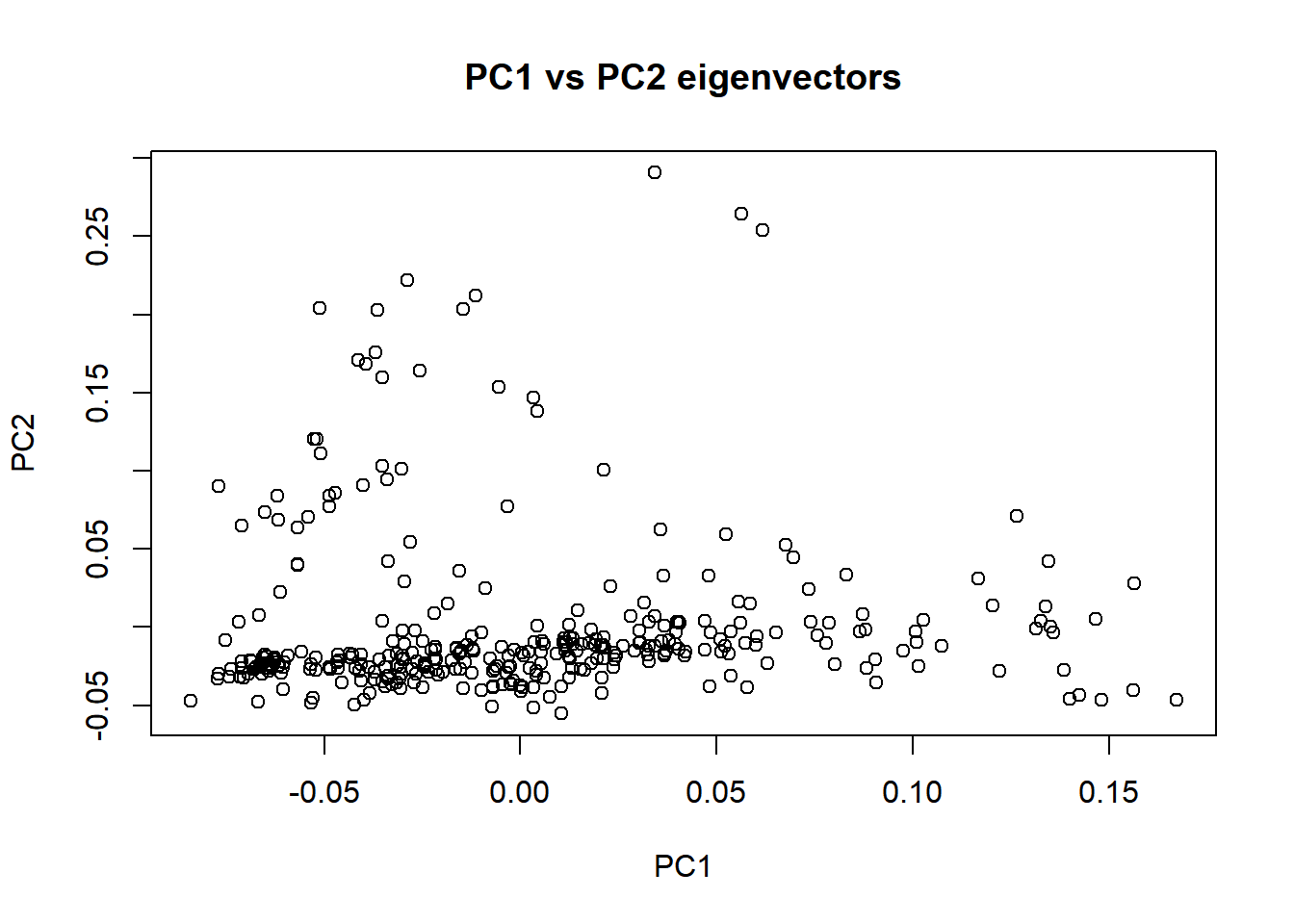

plot(nies_eigenvec071118$V4, nies_eigenvec071118$V5, xlab = "PC2", ylab = "PC3", main = "PC2 vs PC3 eigenvectors")

plot(nies_eigenvec071118$V5, nies_eigenvec071118$V6, xlab = "PC3", ylab = "PC4", main = "PC3 vs PC4 eigenvectors")

Interestingly, the clustering of individuals that was observed in the previous PCA (without filtering for MAF) remained consistent for the PC1 vs PC2 plot.

Removing low frequency and rare variants did not seem to have a significant effect on the PCA results. The plots are still suggestive of population stratification most likely due to the genetic admixture.

Excluding low frequency variants and genomic PCA