| tags: [ Gaston GCTA Genomic Data GREML Heritability ] categories: [Coding Experiments ]
Adding age and sex as covariates
require(magicfor)## Loading required package: magicforrequire(magrittr)## Loading required package: magrittrrequire(dplyr)## Loading required package: dplyr##
## Attaching package: 'dplyr'## The following objects are masked from 'package:stats':
##
## filter, lag## The following objects are masked from 'package:base':
##
## intersect, setdiff, setequal, unionrequire(gaston)## Loading required package: gaston## Loading required package: Rcpp## Loading required package: RcppParallel##
## Attaching package: 'RcppParallel'## The following object is masked from 'package:Rcpp':
##
## LdFlags## Gaston set number of threads to 2. Use setThreadOptions() to modify this.##
## Attaching package: 'gaston'## The following object is masked from 'package:stats':
##
## sigma## The following objects are masked from 'package:base':
##
## cbind, rbindrequire(qqman)## Loading required package: qqman## ## For example usage please run: vignette('qqman')## ## Citation appreciated but not required:## Turner, S.D. qqman: an R package for visualizing GWAS results using Q-Q and manhattan plots. biorXiv DOI: 10.1101/005165 (2014).## ##
## Attaching package: 'qqman'## The following object is masked from 'package:gaston':
##
## manhattanIntroduction
The QQ plots indicate that the GWAS results may be inflated. Typically, this inflation is observed because of population structure, an underpowered study, applying the wrong statistical test, or other hidden factors. I have corrected for population structure by including two principal components, the thresholds applied to the analyses are based on this specific population, and a stringent test is applied to the data set. Therefore, most probable causes for inflation have been accounted for. However, we have not included age and sex as covariates in these analyses because we had concerns about over burdening the model and potentially missing true associations. However, in light of these QQ plots, I will include age and sex as covariates to ensure that the results inflation are not due to these factors.
Methods and Results
Load data
NIES_master <- read.csv('C:/Users/Martha/Documents/Honours/Project/honours.project/Data/NIES_master_database-age.csv', header = T)
covar_col <- c("UUID", "Gender", "Age.excel")
nies_master_covar <- NIES_master[covar_col]

nies_heritable_pheno <- read.csv('C:/Users/Martha/Documents/Honours/Project/honours.project/Data/nies_heritable_pheno.csv', header = T)

nies_heritable_pheno220918 <-read.csv('C:/Users/Martha/Documents/Honours/Project/honours.project/Data/nies_heritable_pheno220918.csv', header = TRUE)

nies_pheno_020918 <- read.csv('C:/Users/Martha/Documents/Honours/Project/honours.project/Data/nies_pheno_020918.csv', header = T)

nies_final_uuid <- nies_heritable_pheno$UUID

nies_covar <- nies_master_covar[nies_master_covar$UUID %in% nies_final_uuid,]
nies_covar <- as.matrix(nies_covar)


merged_nies_210818 <- read.bed.matrix("C:/Users/Martha/Documents/Honours/Project/honours.project/Data/merged_nies/merged_nies_geno_210818.bed")
## Reading C:/Users/Martha/Documents/Honours/Project/honours.project/Data/merged_nies/merged_nies_geno_210818.fam
## Reading C:/Users/Martha/Documents/Honours/Project/honours.project/Data/merged_nies/merged_nies_geno_210818.bim
## Reading C:/Users/Martha/Documents/Honours/Project/honours.project/Data/merged_nies/merged_nies_geno_210818.bed
## ped stats and snps stats have been set.
## 'p' has been set.
## 'mu' and 'sigma' have been set.merged_nies_GRM <- GRM(merged_nies_210818)
merged_nies_eiK <- eigen(merged_nies_GRM)
merged_nies_eiK$values[ merged_nies_eiK$values < 0] <- 0
merged_nies_PC <- sweep(merged_nies_eiK$vectors, 2, sqrt(merged_nies_eiK$values), "*")1. Heritability analyses in GCTA
for i in {1..27}
do ./gcta64 --reml --grm gcta_output/merged_nies_grm --pheno nies_pheno_020918.txt --mpheno $i --reml-pred-rand --covar nies_sex_covar.txt --qcovar nies_pca_age_covar.txt --out gcta_output/$i.covar.est
head gcta_output/$i.covar.est.hsq >> trait.her.covar.gcta.txt
done

for i in {1..9}
do ./gcta64 --reml --grm gcta_output/merged_nies_grm --pheno pheno_pca_coord.txt --mpheno $i --reml-pred-rand --covar nies_sex_covar.txt --qcovar nies_pca_age_covar.txt --out gcta_output/$i.pc.covar.est
head gcta_output/$i.pc.covar.est.hsq >> pc.her.covar.gcta.txt
done
heritability_covar_gcta <- read.csv('C:/Users/Martha/Documents/Honours/Project/honours.project/Data/heritability_covar_gcta2.csv', header = TRUE)
heritability_covar_gcta## Trait h2 pval X PC h2.1 pval.1 X.1
## 1 R.K.value.V 0.732774 1.68e-07 NA 1 0.584877 1.47e-05 NA
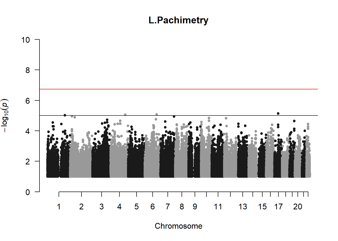
## 2 L.Pachimetry 0.672052 4.45e-07 NA 4 0.473562 9.97e-05 NA
## 3 R.Pachimetry 0.622011 2.47e-06 NA 3 0.315501 5.14e-03 NA
## 4 R.Cyl..pre.dilate. 0.595018 1.55e-06 NA 8 0.193069 2.94e-02 NA
## 5 totaluvafmm 0.594148 2.06e-05 NA 7 0.239878 3.69e-02 NA
## 6 R.CDR 0.590256 3.34e-05 NA 2 0.262234 5.35e-02 NA
## 7 L.K.value.V 0.570662 2.97e-05 NA NA NA NA NA
## 8 R.K.value.H 0.500294 1.17e-04 NA 6 0.136592 1.32e-01 NA
## 9 L.CDR 0.496006 7.02e-04 NA 9 0.006853 4.77e-01 NA
## 10 L.Axial.Length 0.336035 6.72e-03 NA 5 0.000000 5.00e-01 NA
## 11 R.Axial.Length 0.324886 8.16e-03 NA NA NA NA NA
## 12 L.K.value.H 0.285803 2.55e-02 NA NA NA NA NA
## 13 R.AC.Depth 0.267335 1.09e-02 NA NA NA NA NA
## 14 L.AC.Depth 0.266877 1.08e-02 NA NA NA NA NA
## 15 R.IOP.mmHg 0.244349 3.13e-02 NA NA NA NA NA
## 16 L.IOP.mmHg 0.205074 4.58e-02 NA NA NA NA NA
## 17 L.Axis..pre.dilate. 0.115745 1.96e-01 NA NA NA NA NA
## 18 R.Axis..pre.dilate. 0.038499 3.92e-01 NA NA NA NA NA
## 19 R.Logmar.VA 0.000000 5.00e-01 NA NA NA NA NA
## 20 L.Logmar.VA 0.000000 5.00e-01 NA NA NA NA NA
## 21 R.Sph..pre.dilate. 0.000000 5.00e-01 NA NA NA NA NA
## 22 L.Sph..pre.dilate. 0.000000 5.00e-01 NA NA NA NA NA
## 23 L.Cyl..pre.dilate. 0.000000 5.00e-01 NA NA NA NA NA
## 24 R.K.Value.H.Axis 0.000000 5.00e-01 NA NA NA NA NA
## 25 R.K.value.V.Axis 0.000000 5.00e-01 NA NA NA NA NA
## 26 L.K.value.H.Axis 0.000000 5.00e-01 NA NA NA NA NA
## 27 L.K.value.V.Axis 0.000000 5.00e-01 NA NA NA NA NA
## X.2 X.3
## 1 cct 0.6470315
## 2 kvalue 0.5220000
## 3 cdr 0.5431310
## 4 ax length 0.3304605
## 5 acd 0.2671060
## 6 iop 0.2247115
## 7 UVAF 0.5900000
## 8 NA
## 9 NA
## 10 NA
## 11 NA
## 12 NA
## 13 NA
## 14 NA
## 15 NA
## 16 NA
## 17 NA
## 18 NA
## 19 NA
## 20 NA
## 21 NA
## 22 NA
## 23 NA
## 24 NA
## 25 NA
## 26 NA
## 27 NAThese heritability estimates differ from the previous estimates suggesting that sex and age have a significant influence on the outcome of the analyses. All traits that are statistically significant (p < 0.05) will be prioritised for pedigree-based GWAS.
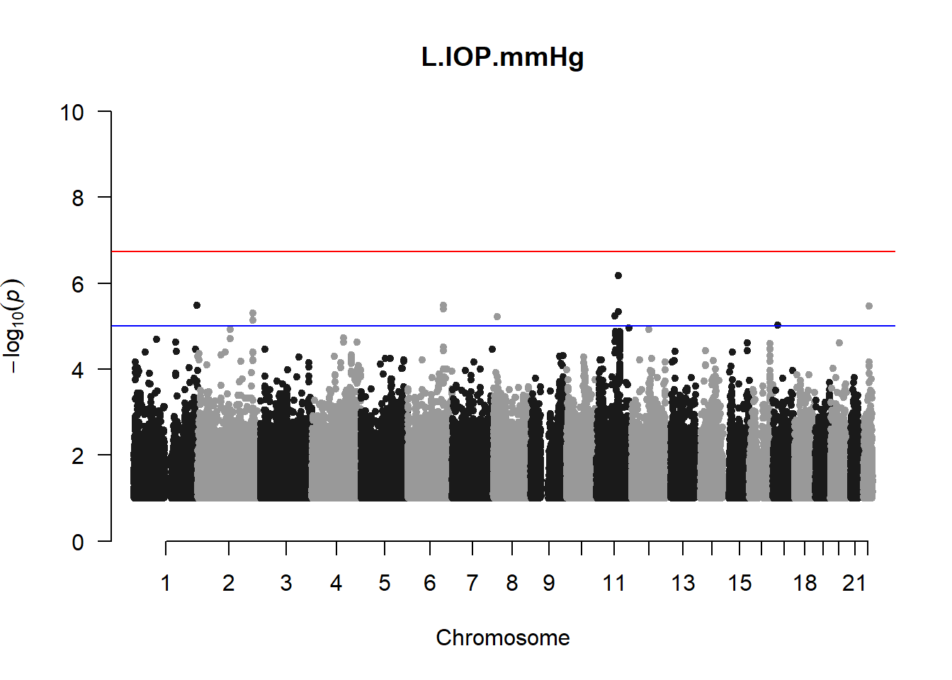
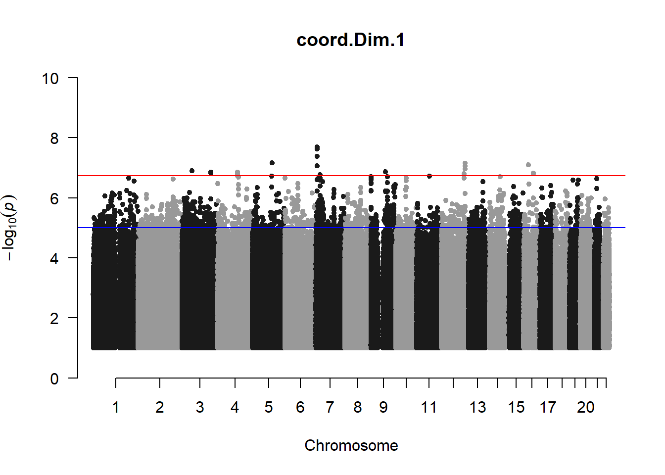
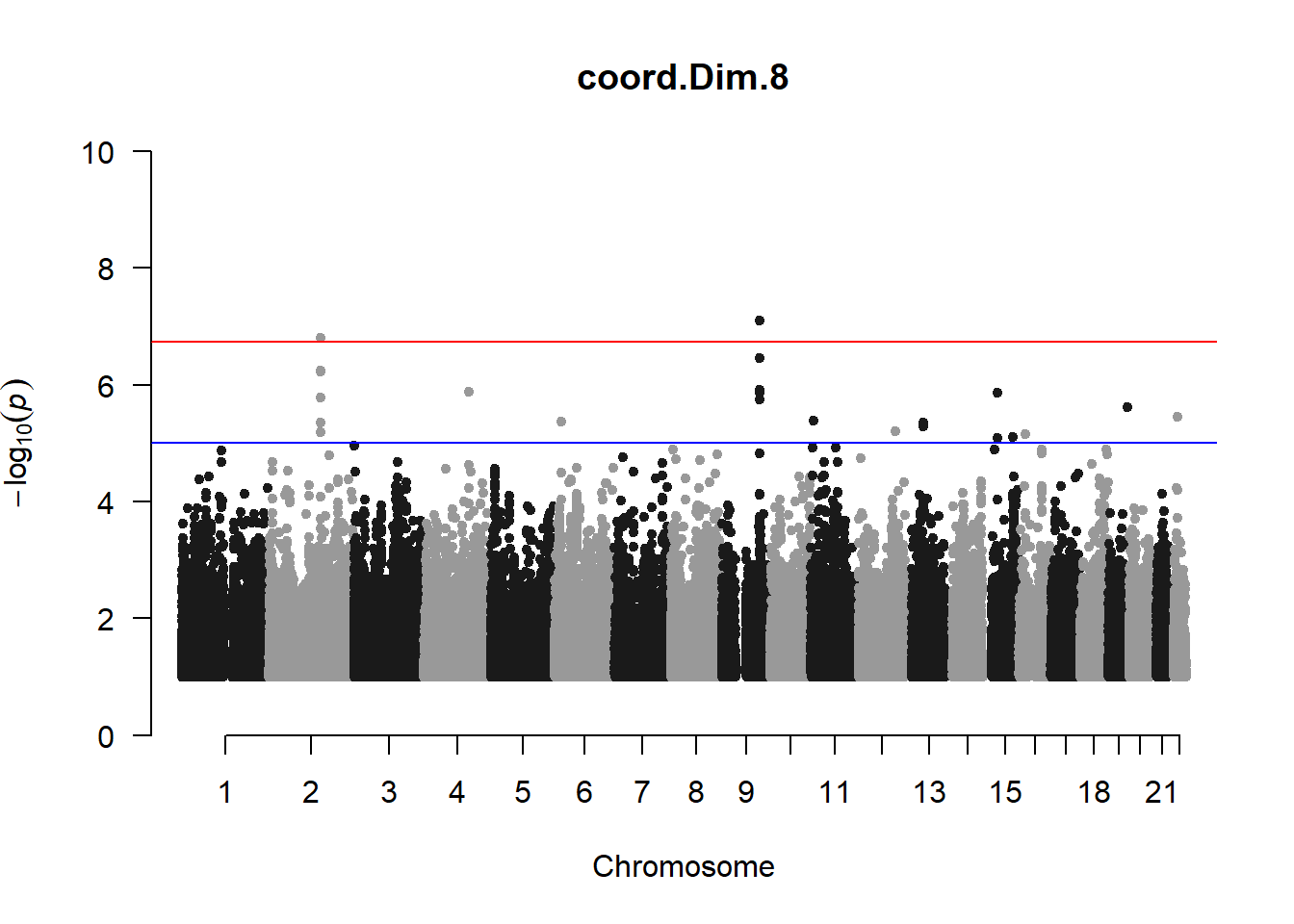
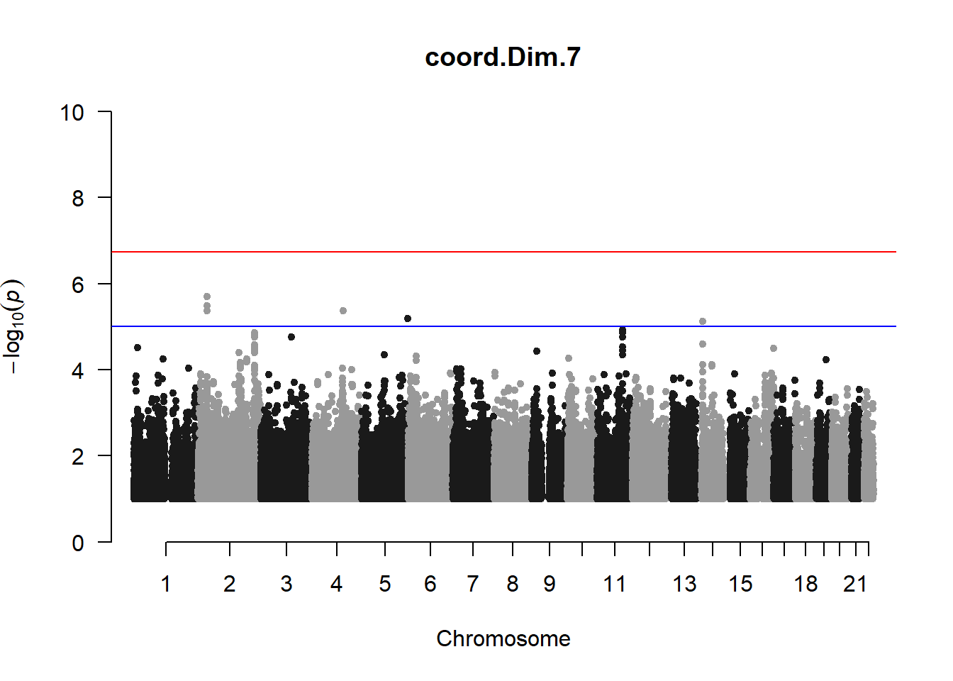
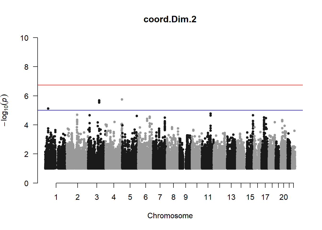
2. Perform GWAS using lmm and LRT
nies_covar <- read.csv('C:/Users/Martha/Documents/Honours/Project/honours.project/Data/nies_covar.csv', header =T)
nies_heritable_pheno240918 <- read.csv('C:/Users/Martha/Documents/Honours/Project/honours.project/Data/nies_heritable_pheno240918.csv', header = TRUE)

for (i in c(2:ncol(nies_heritable_pheno240918))){
  pheno_colnames <- colnames(nies_heritable_pheno240918[i])
  her_pheno_gwas <- association.test(merged_nies_210818, nies_heritable_pheno240918[,i], X = nies_covar, method = "lmm", test = "lrt", K = merged_nies_GRM, eigenK = merged_nies_eiK, p =2)
  her_pheno_gwas <- na.omit(her_pheno_gwas)
  pheno_gwas_filtered <- her_pheno_gwas %>% filter(-log10(p)>1) %>% filter(freqA2 < 0.99)
  qqman::manhattan(x = pheno_gwas_filtered, chr = "chr", bp = "pos", p = "p", snp = "id", genomewideline = -log10(1.84e-7), main = paste(pheno_colnames), ylim = c(0,10))
}
## Warning in trans.X(X, eigenK$vectors[, seq_len(p)], mean(Y)): An intercept
## column was added to the covariate matrix X
## Warning in trans.X(X, eigenK$vectors[, seq_len(p)], mean(Y)): An intercept
## column was added to the covariate matrix X

## Warning in trans.X(X, eigenK$vectors[, seq_len(p)], mean(Y)): An intercept
## column was added to the covariate matrix X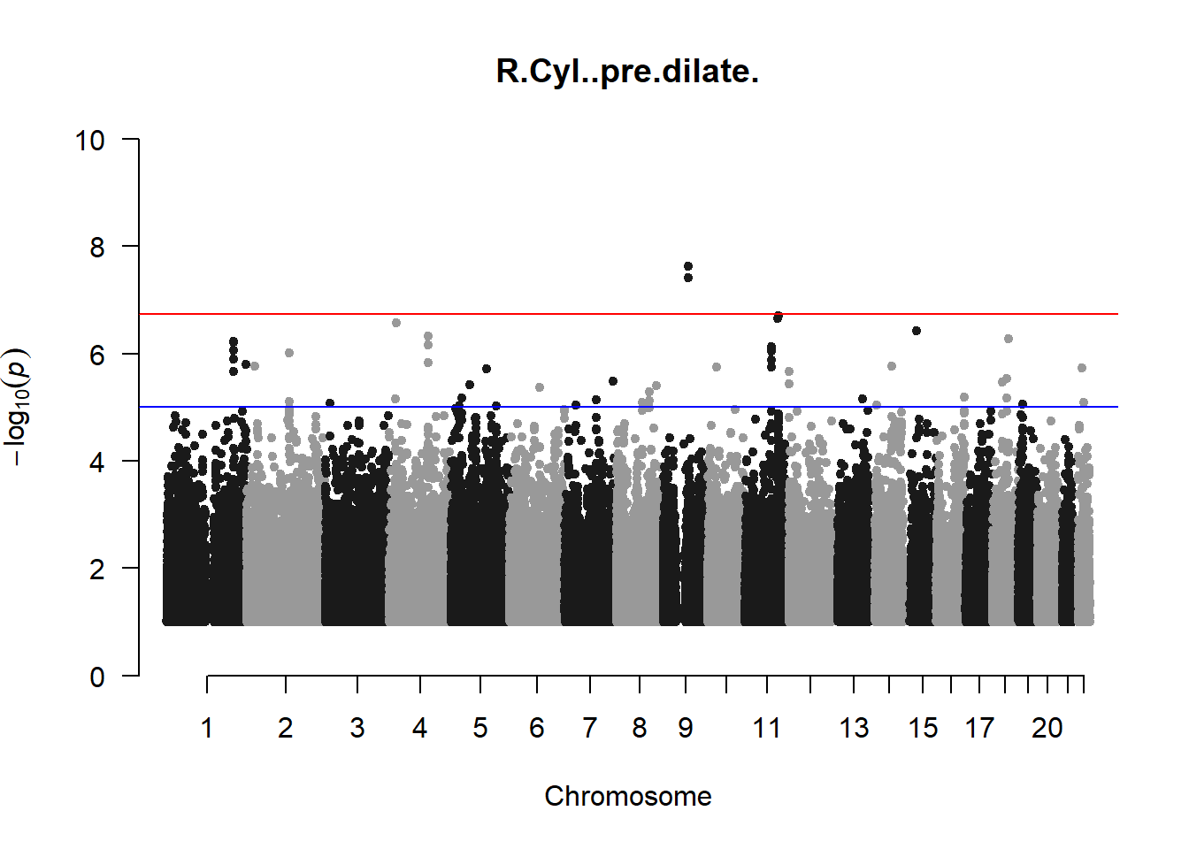
## Warning in trans.X(X, eigenK$vectors[, seq_len(p)], mean(Y)): An intercept
## column was added to the covariate matrix X
## Warning in trans.X(X, eigenK$vectors[, seq_len(p)], mean(Y)): An intercept
## column was added to the covariate matrix X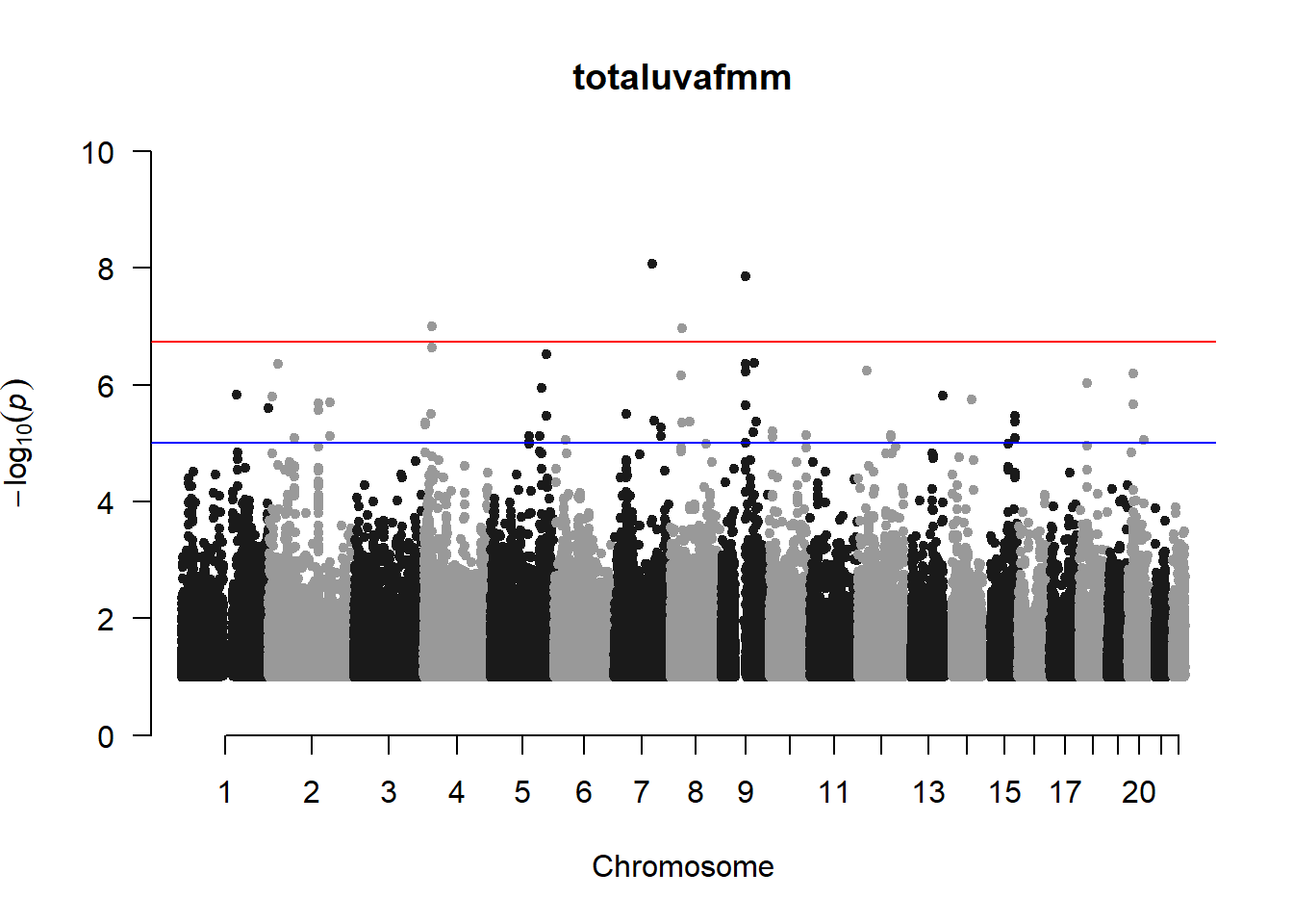
## Warning in trans.X(X, eigenK$vectors[, seq_len(p)], mean(Y)): An intercept
## column was added to the covariate matrix X
## Warning in trans.X(X, eigenK$vectors[, seq_len(p)], mean(Y)): An intercept
## column was added to the covariate matrix X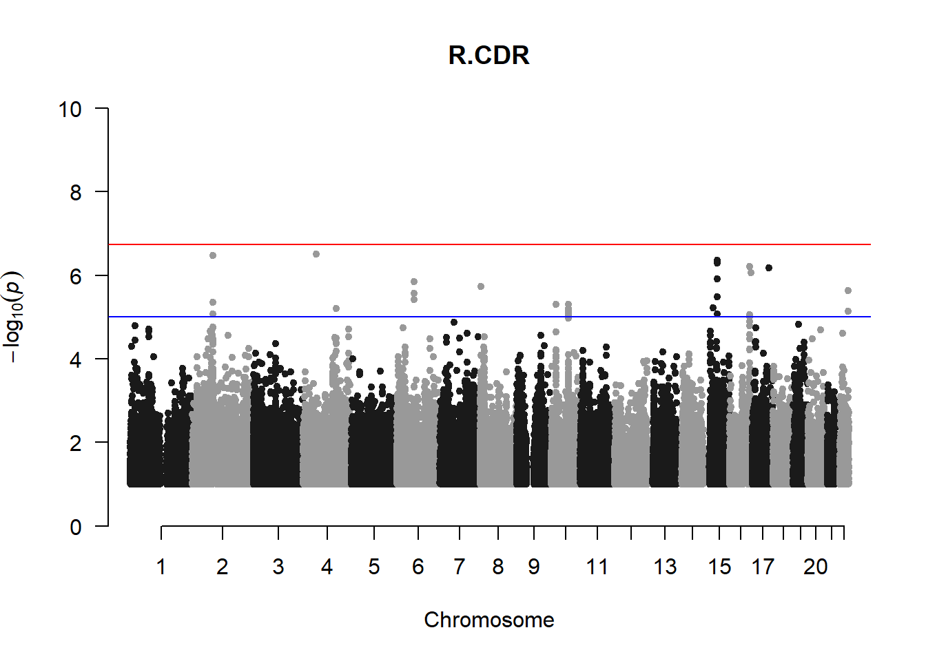
## Warning in trans.X(X, eigenK$vectors[, seq_len(p)], mean(Y)): An intercept
## column was added to the covariate matrix X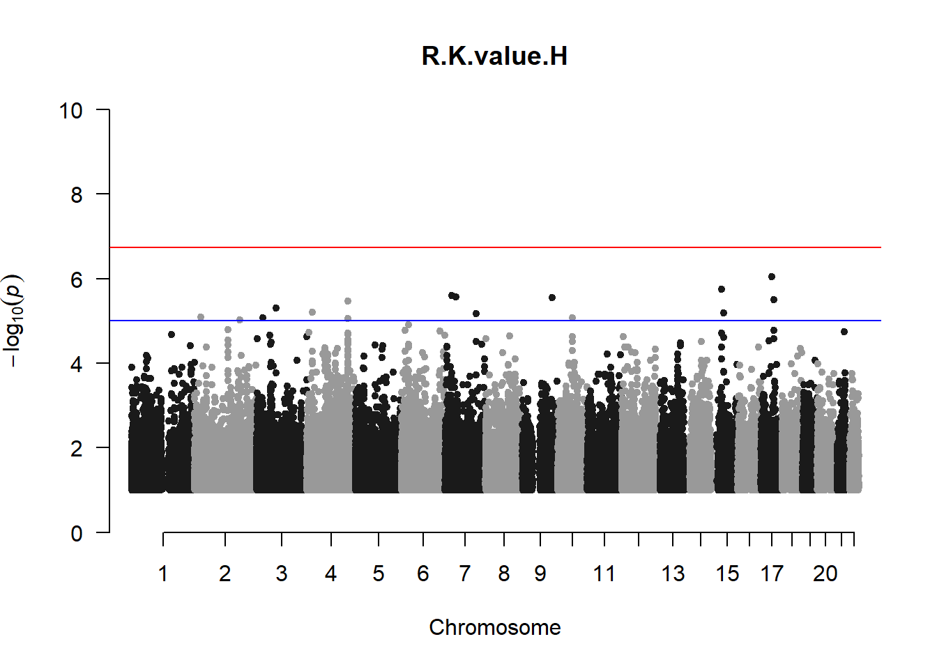
## Warning in trans.X(X, eigenK$vectors[, seq_len(p)], mean(Y)): An intercept
## column was added to the covariate matrix X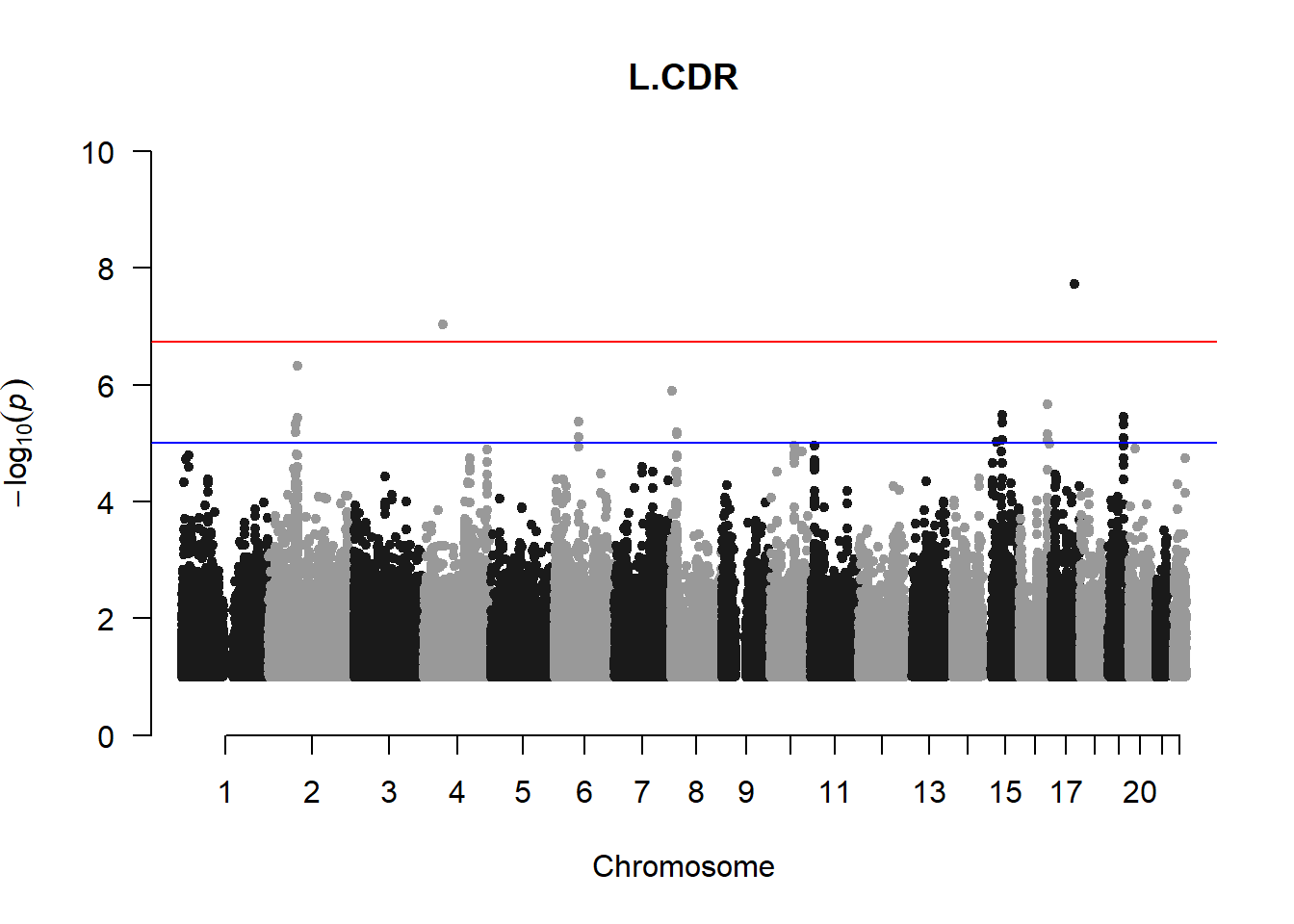
## Warning in trans.X(X, eigenK$vectors[, seq_len(p)], mean(Y)): An intercept
## column was added to the covariate matrix X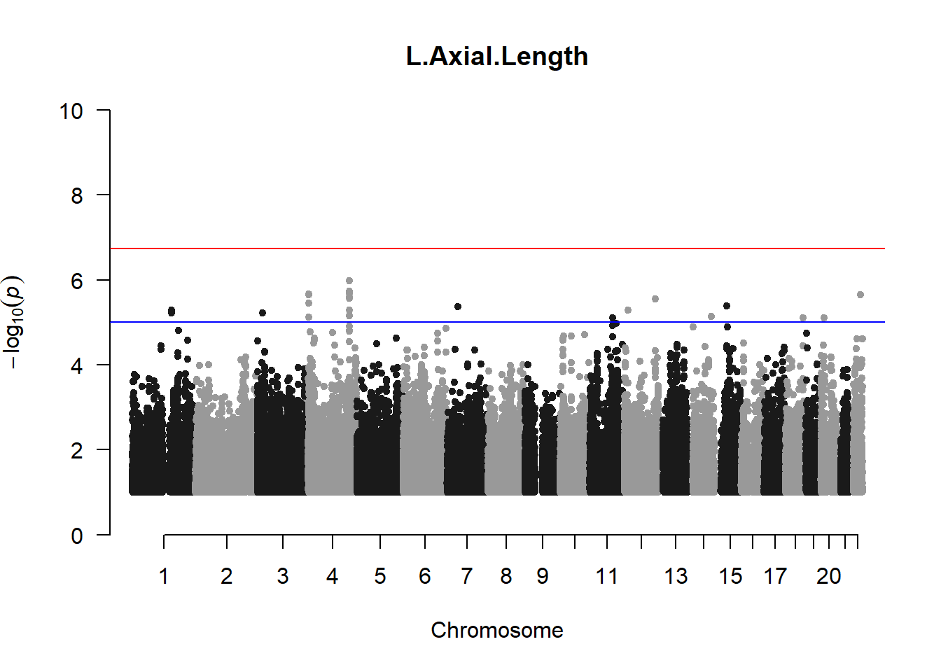
## Warning in trans.X(X, eigenK$vectors[, seq_len(p)], mean(Y)): An intercept
## column was added to the covariate matrix X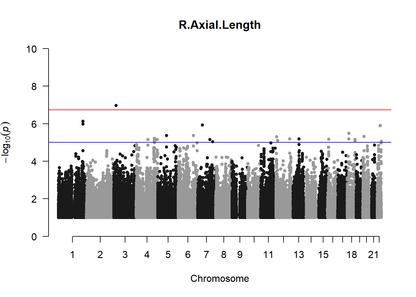
## Warning in trans.X(X, eigenK$vectors[, seq_len(p)], mean(Y)): An intercept
## column was added to the covariate matrix X
## Warning in trans.X(X, eigenK$vectors[, seq_len(p)], mean(Y)): An intercept
## column was added to the covariate matrix X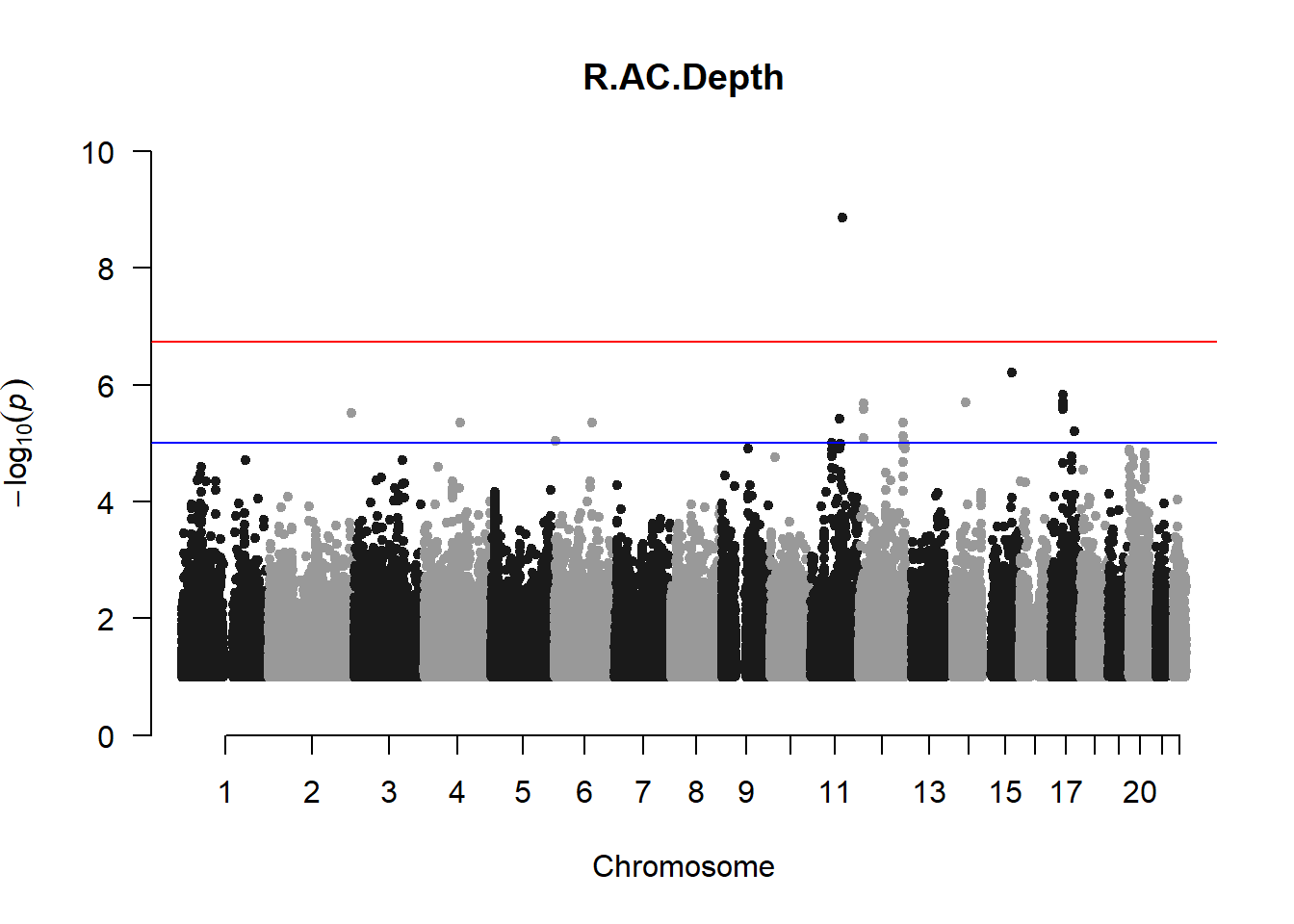
## Warning in trans.X(X, eigenK$vectors[, seq_len(p)], mean(Y)): An intercept
## column was added to the covariate matrix X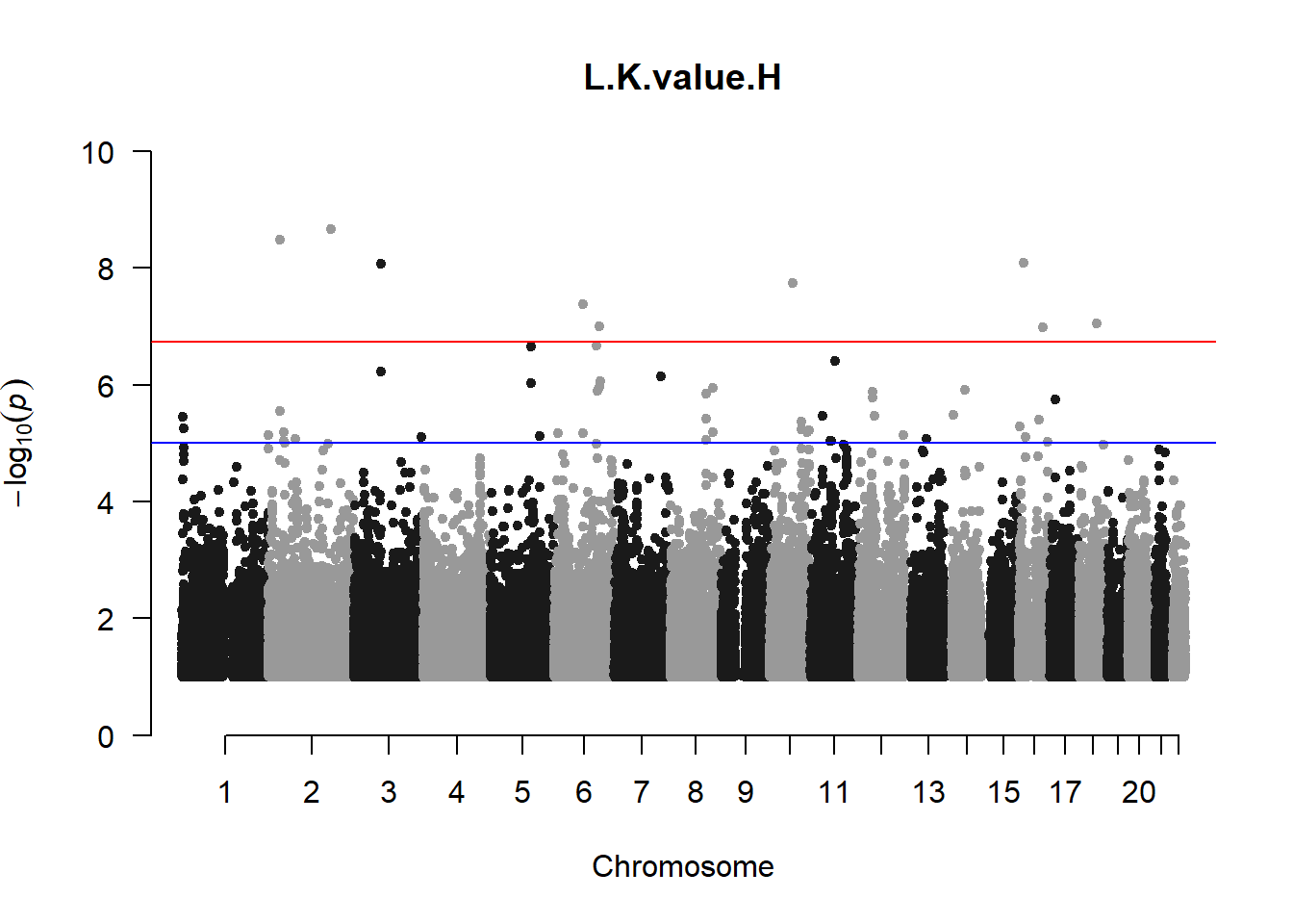
## Warning in trans.X(X, eigenK$vectors[, seq_len(p)], mean(Y)): An intercept
## column was added to the covariate matrix X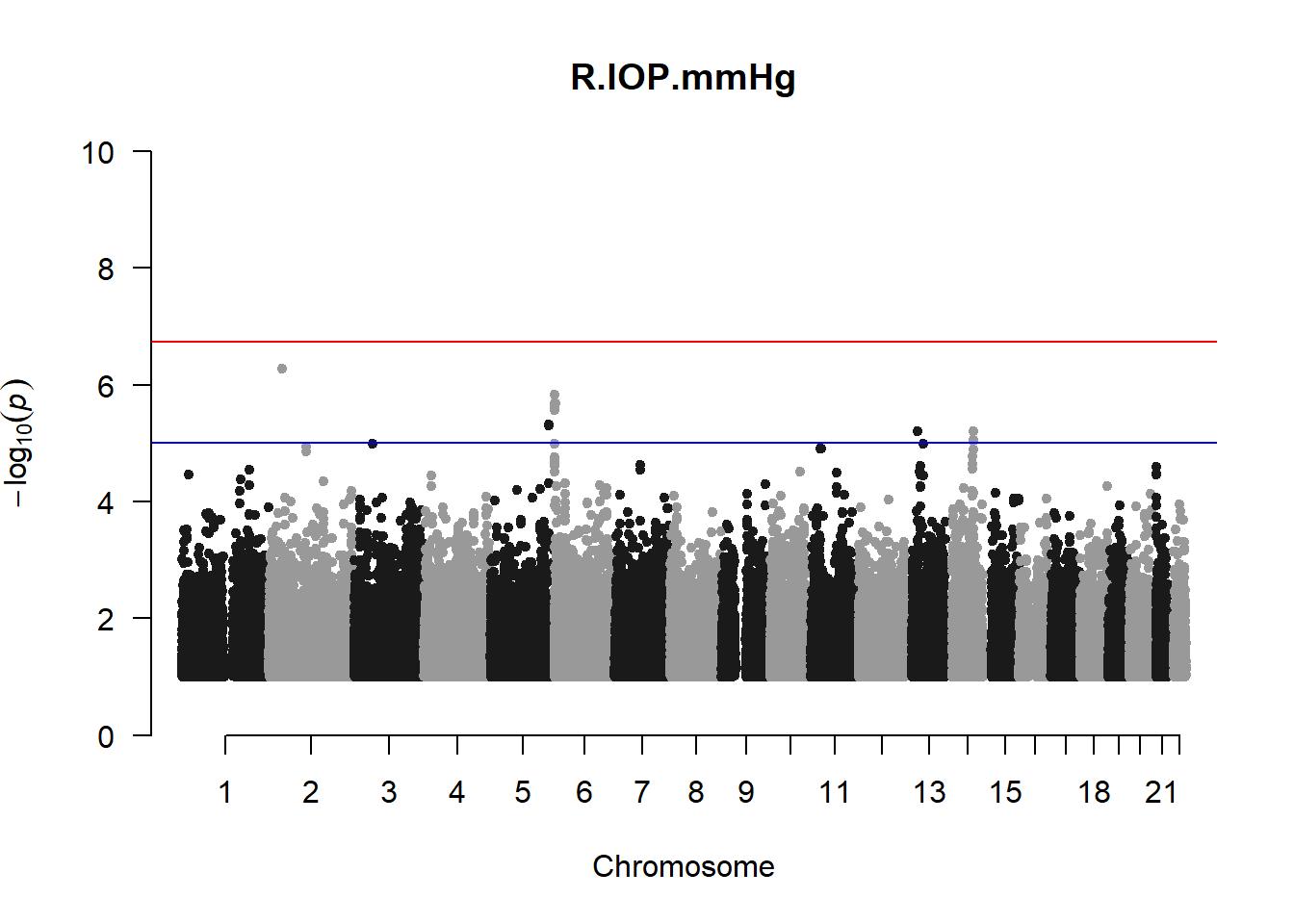
## Warning in trans.X(X, eigenK$vectors[, seq_len(p)], mean(Y)): An intercept
## column was added to the covariate matrix X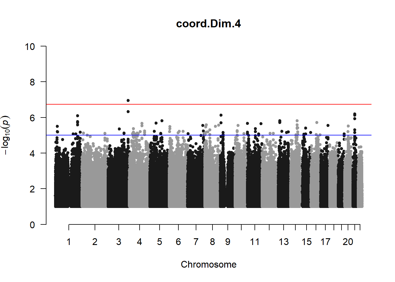
## Warning in trans.X(X, eigenK$vectors[, seq_len(p)], mean(Y)): An intercept
## column was added to the covariate matrix X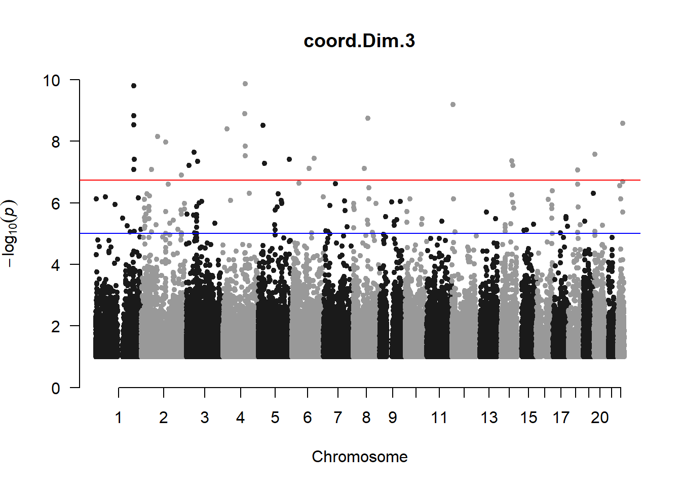
3. Generate QQ plots for GWAS resutls
for (i in c(2:ncol(nies_heritable_pheno240918))){
  pheno_colnames <- colnames(nies_heritable_pheno240918[i])
  her_pheno_gwas <- association.test(merged_nies_210818, nies_heritable_pheno240918[,i], method = "lmm",
                                     test = "lrt", K = merged_nies_GRM, eigenK = merged_nies_eiK, p =2)
  her_pheno_gwas <- na.omit(her_pheno_gwas)
  pheno_gwas_filtered <- her_pheno_gwas  %>% filter(freqA2 < 0.99)
  gaston:: qqplot.pvalues(pheno_gwas_filtered$p, main = paste(pheno_colnames))
}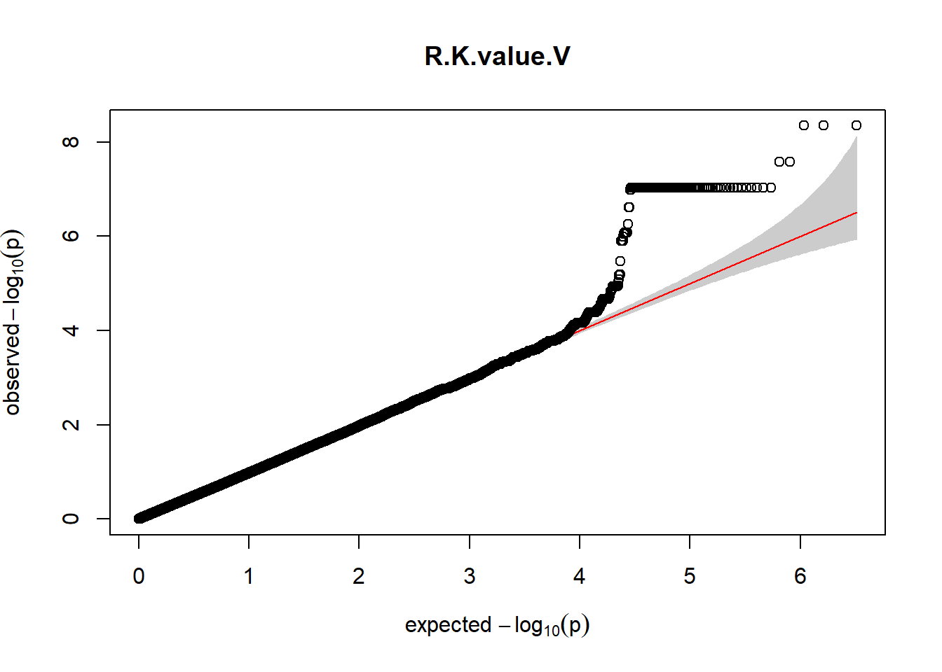
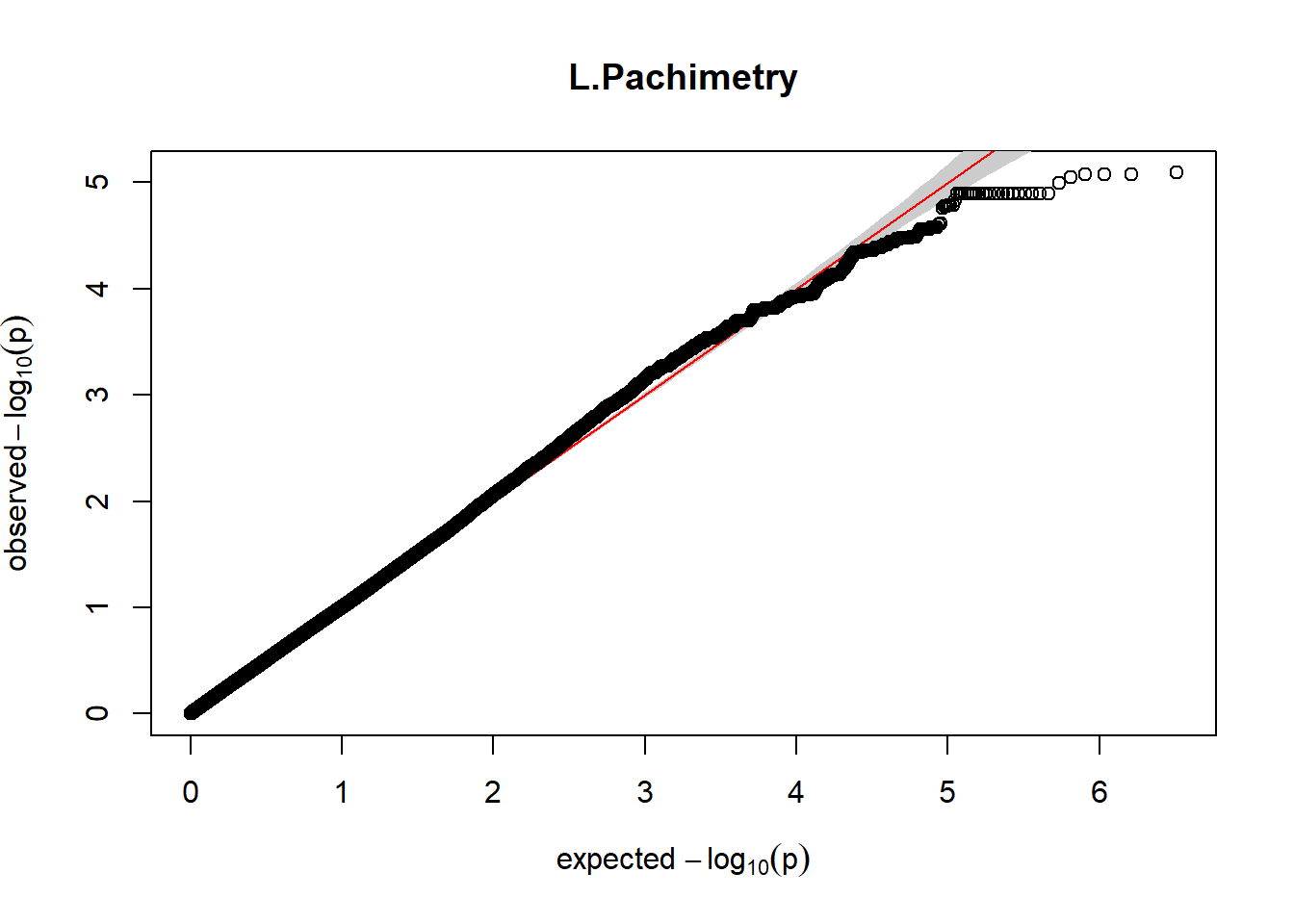
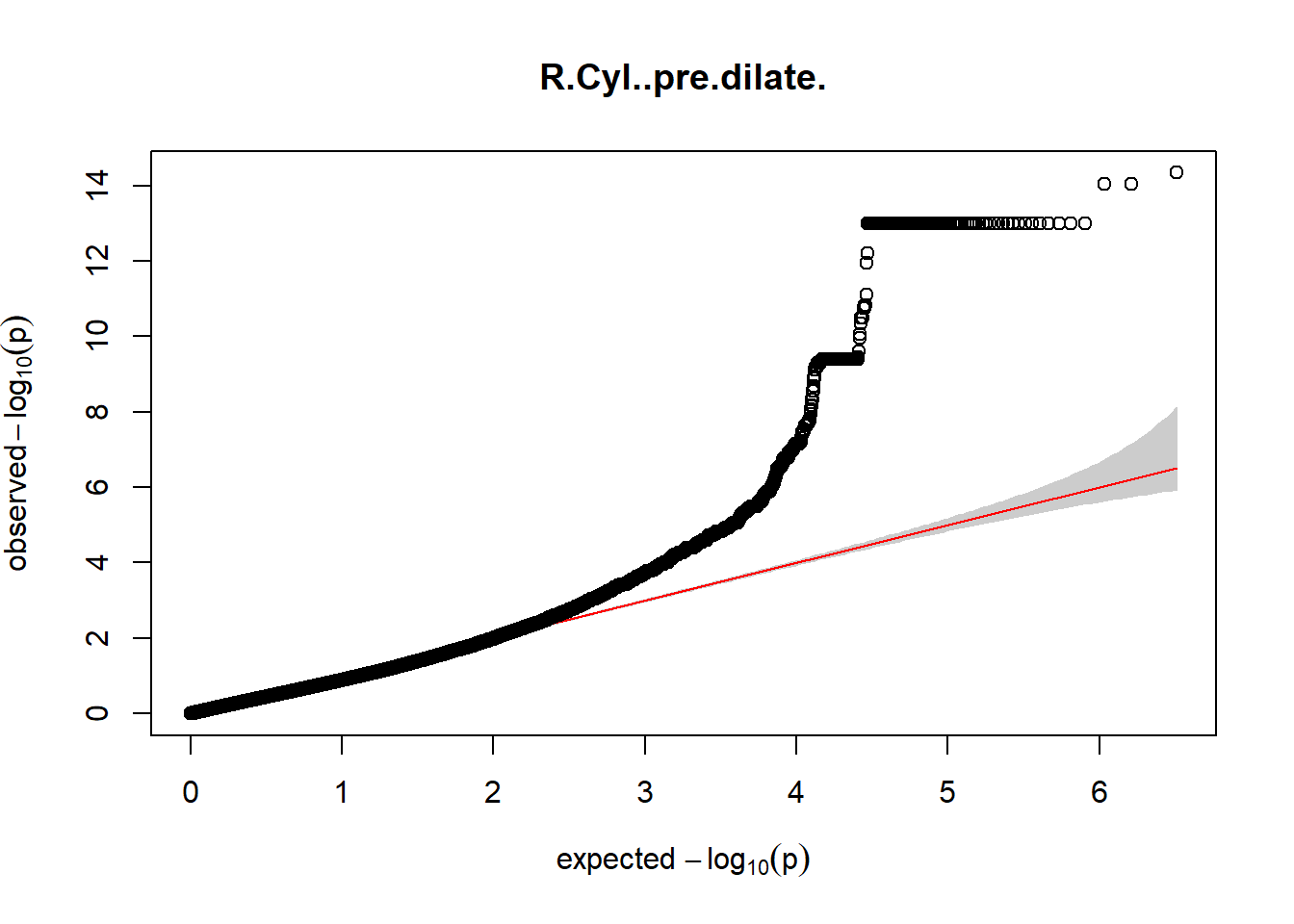
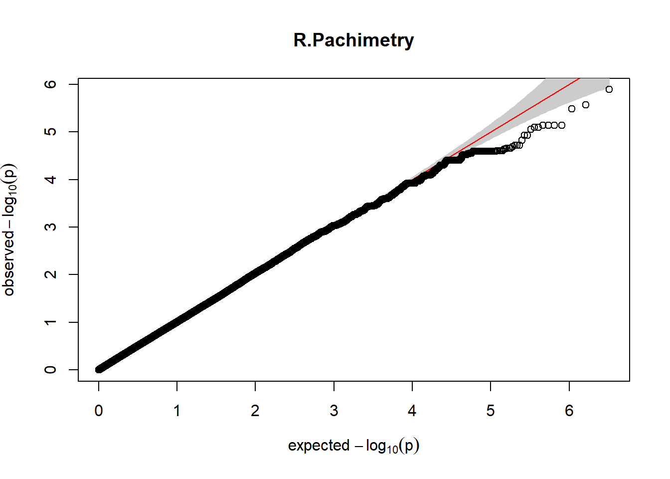
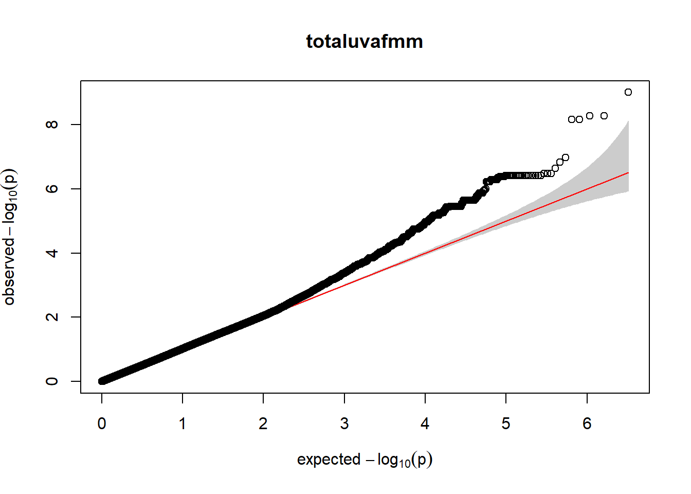
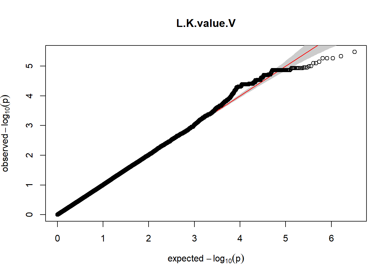
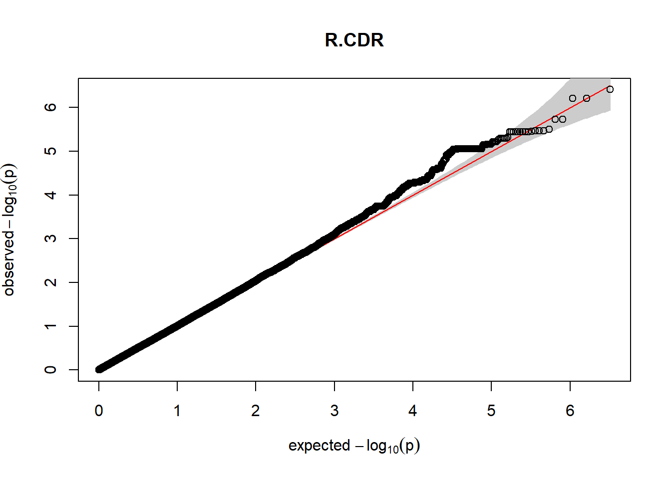
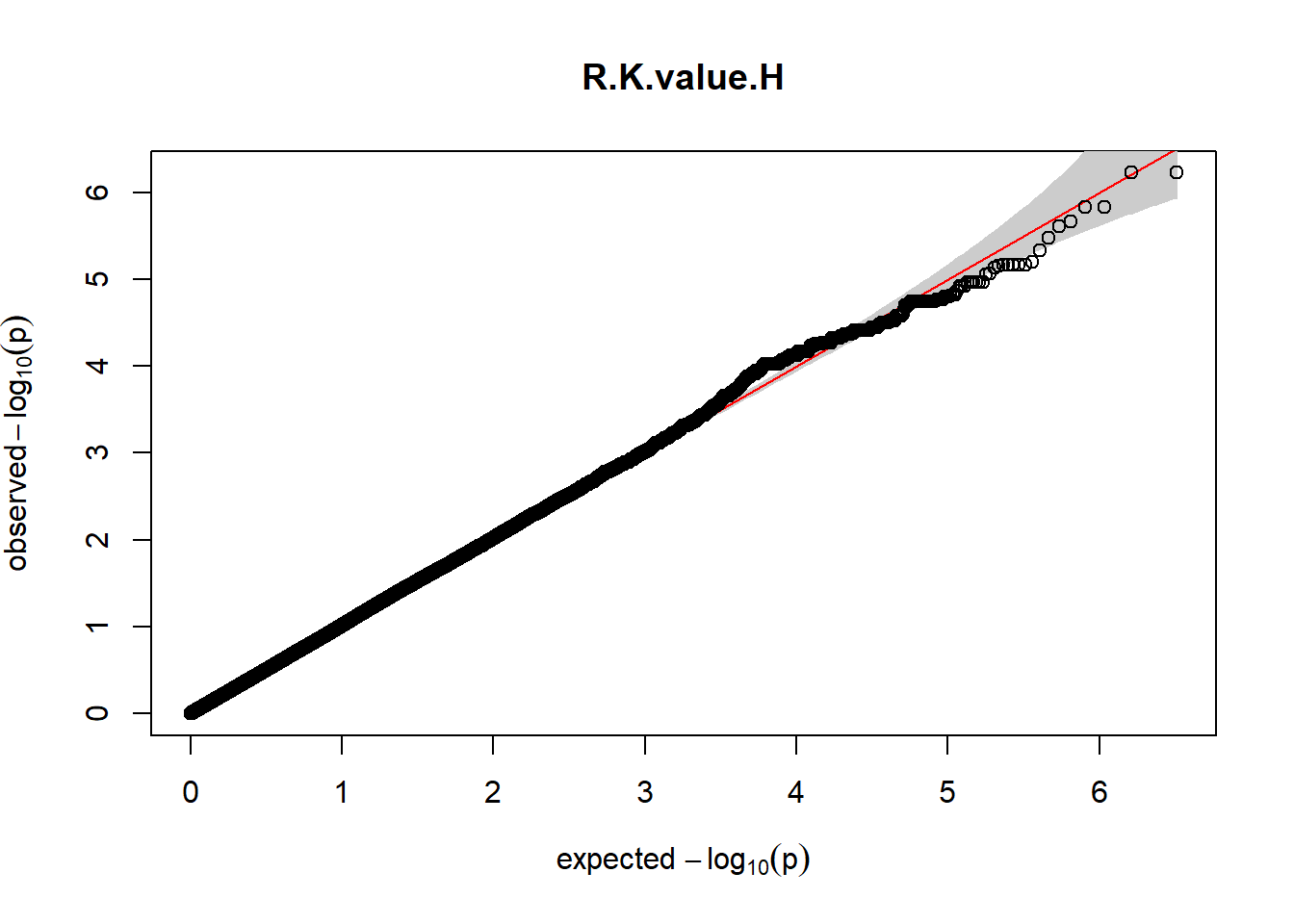
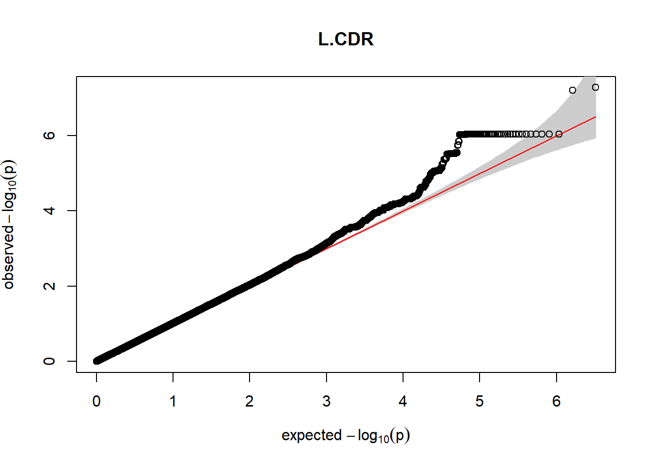
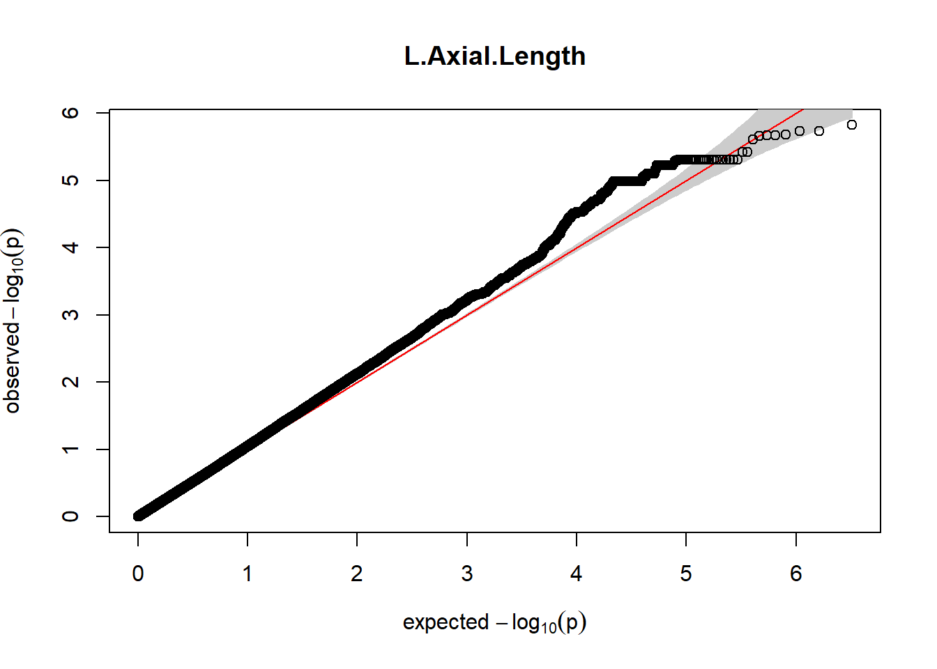
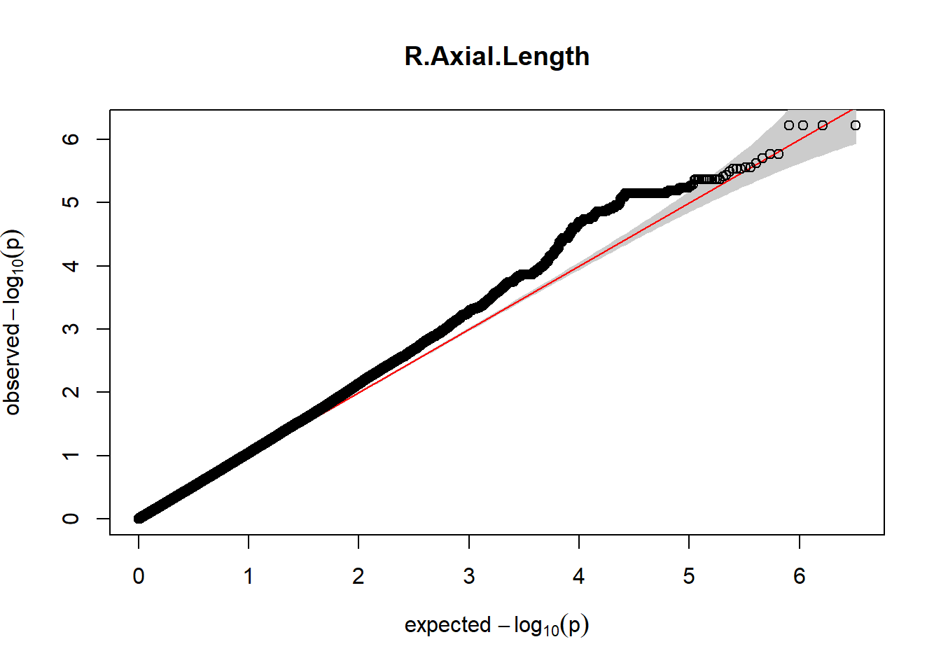
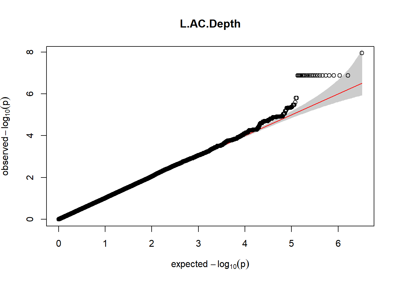
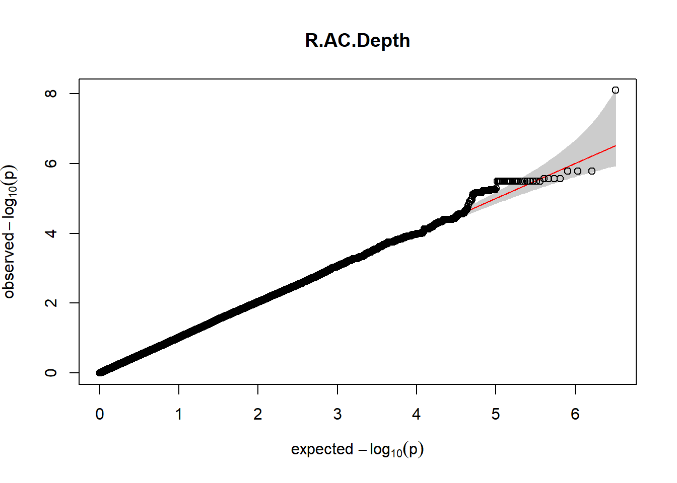
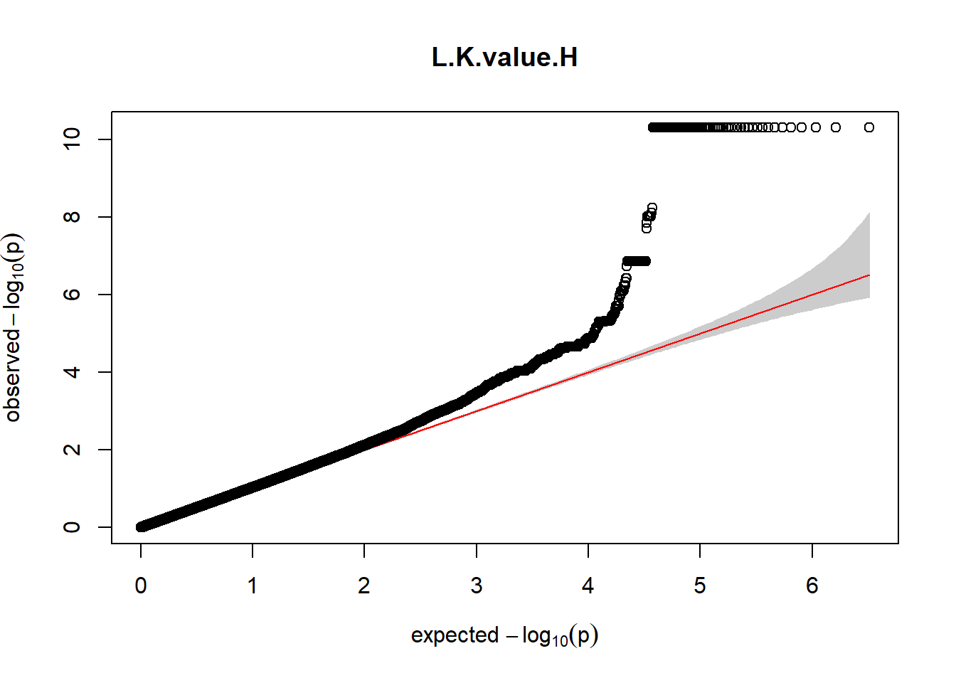
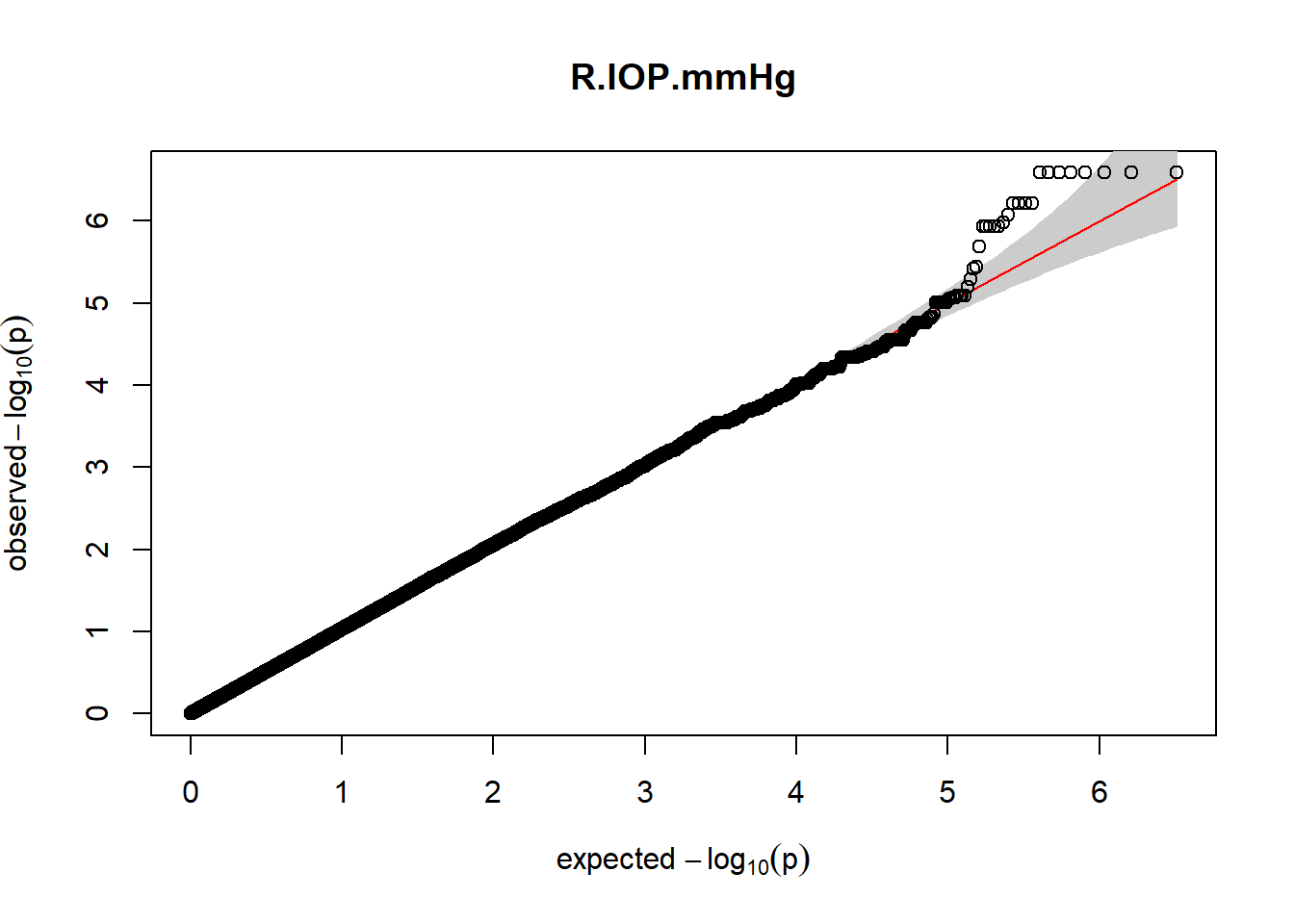
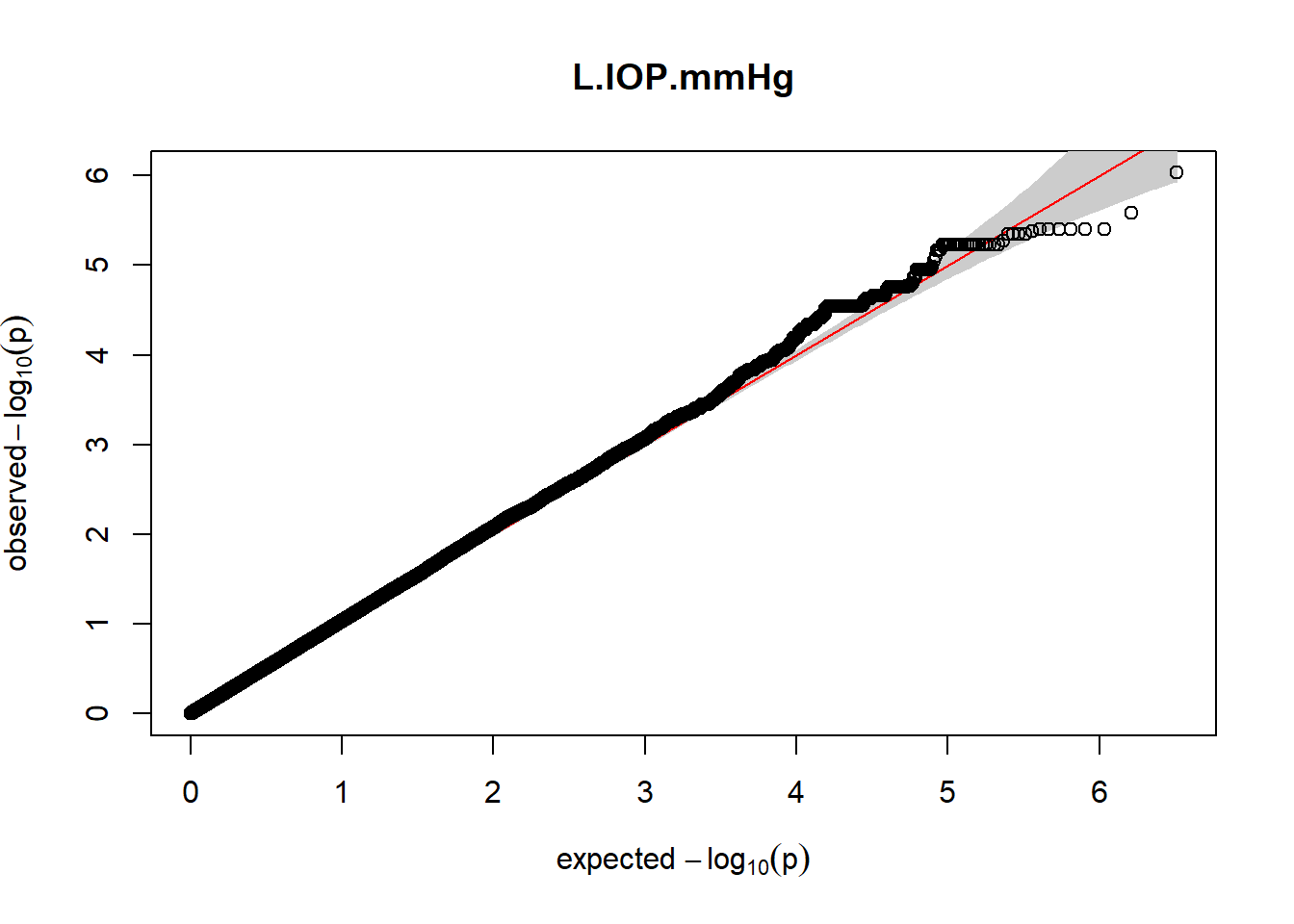

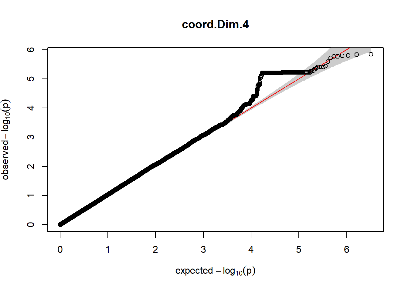
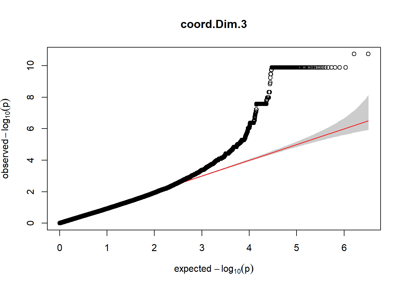
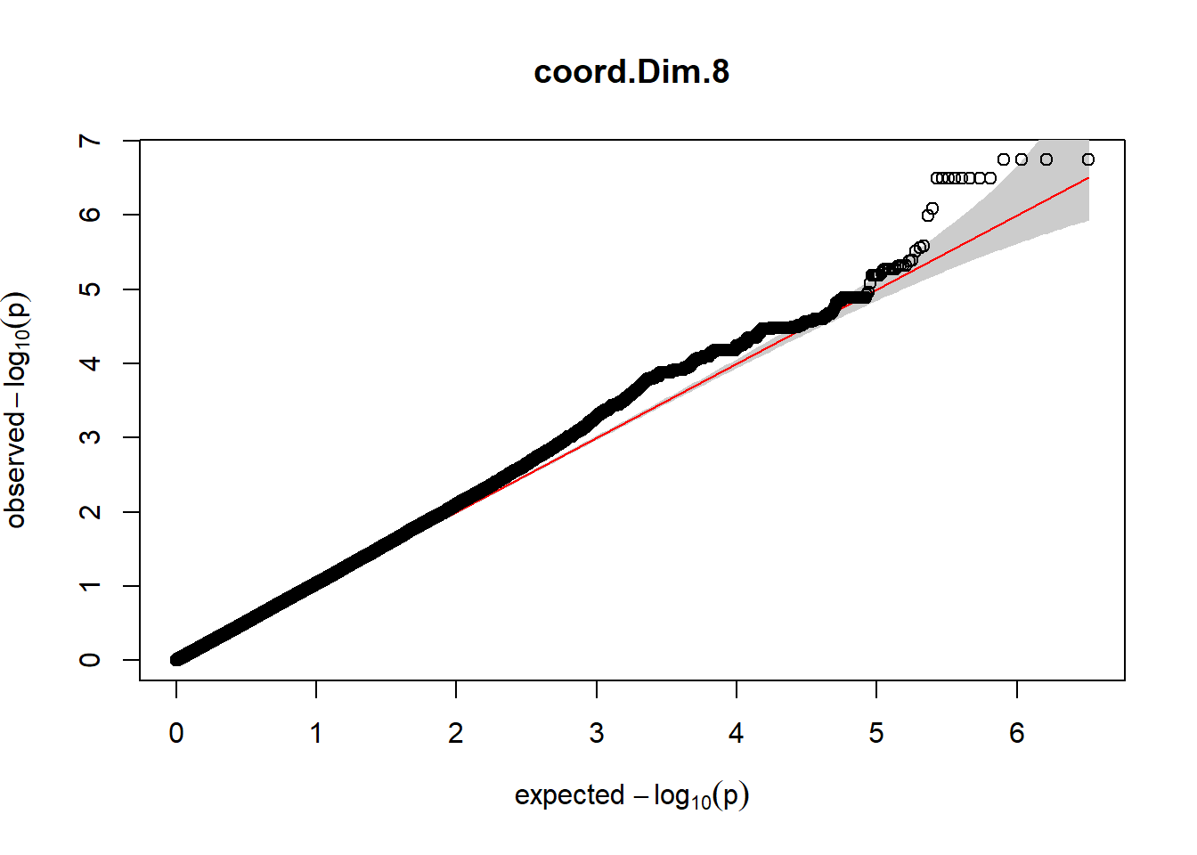
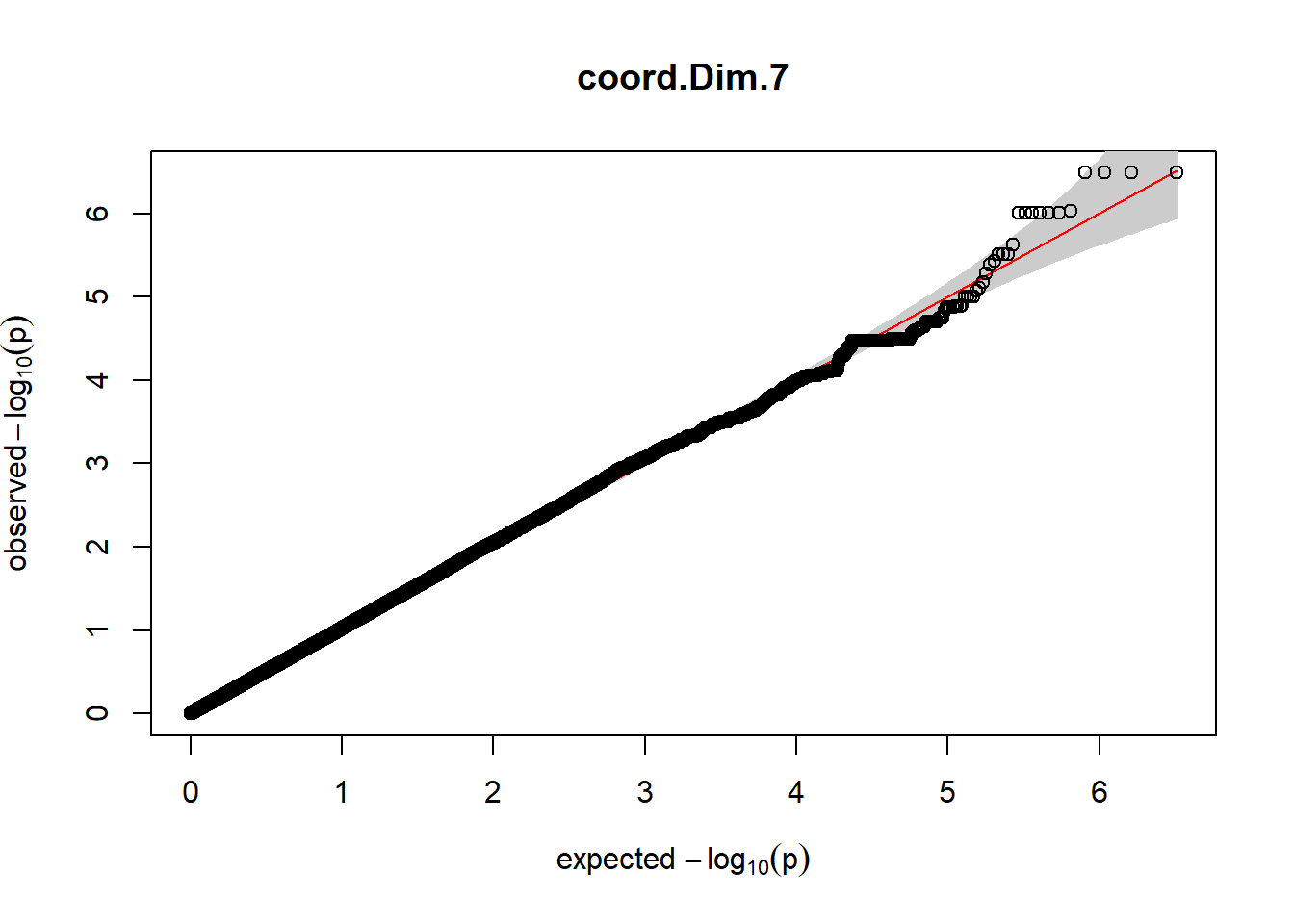
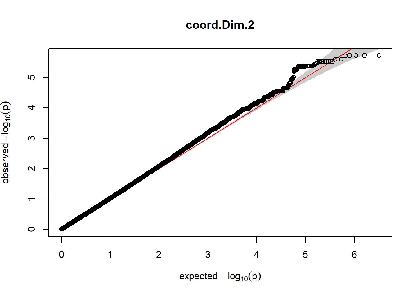
Despite the inclusion of age and sex as covariates, these QQ plots are still indicative of some inflation of the results.