Methods and Results

1. load data

phen.data.age <- read.csv('C:/Users/Martha/Documents/Honours/Project/honours.project/Data/NIES_master_database-age.csv')
phen.data.adults<-phen.data.age[phen.data.age$Age.excel>17,]
quant.variables<- c("R.K.value.H", "R.K.Value.H.Axis", "R.K.value.V", "R.K.value.V.Axis", "L.K.value.H",
                    "L.K.value.H.Axis", "L.K.value.V", "L.K.value.V.Axis", "R.Pachimetry", "L.Pachimetry", "R.Axial.Length",
                    "L.Axial.Length", "AC.Depth.R", "AC.Depth.L", "R.IOP.mmHg", "L.IOP.mmHg", "CDR.RE", "CDR.LE")
quant.data.adults<- phen.data.adults[quant.variables]

2. install relevant packages

install.packages('missMDA', dependencies = TRUE, repos = "http://cran.us.r-project.org")

## Installing package into 'C:/Users/Martha/Documents/R/win-library/3.4'
## (as 'lib' is unspecified)

## package 'missMDA' successfully unpacked and MD5 sums checked
## 
## The downloaded binary packages are in
##  C:\Users\Martha\AppData\Local\Temp\RtmpaopRRl\downloaded_packages

require(missMDA)

## Loading required package: missMDA

require(FactoMineR)

## Loading required package: FactoMineR

3. Estimate the number of dimensions to be used for the reconstruction formula

data(quant.data.adults)

## Warning in data(quant.data.adults): data set 'quant.data.adults' not found

nb = estim_ncpPCA(quant.data.adults)
nb

## $ncp
## [1] 0
## 
## $criterion
##         0         1         2         3         4         5 
##  805.7256  908.9445  966.5074 1029.5131 1088.5948  880.7742

4. Impute the data with the number of dimensions previously calculated

res.comp = imputePCA(quant.data.adults,ncp=nb$ncp)
head(res.comp$completeObs) #view imputed dataset

##   R.K.value.H R.K.Value.H.Axis R.K.value.V R.K.value.V.Axis L.K.value.H
## 1    42.00000          2.00000    43.00000         92.00000    42.50000
## 2    41.25000          7.00000    42.25000         97.00000    41.50000
## 3    42.96687         93.74108    43.79634         91.18098    42.96871
## 4    44.75000          5.00000    45.00000         95.00000    45.00000
## 5    44.75000          0.00000    44.75000         90.00000    44.25000
## 6    42.00000          8.00000    43.25000         98.00000    42.25000
##   L.K.value.H.Axis L.K.value.V L.K.value.V.Axis R.Pachimetry L.Pachimetry
## 1          5.00000    43.50000         95.00000          532          554
## 2        168.00000    42.00000         78.00000          608          612
## 3         87.79947    43.87197         92.21768          507          510
## 4         60.00000    45.25000        150.00000          560          559
## 5        178.00000    44.75000         88.00000          556          562
## 6        177.00000    43.25000         87.00000          498          501
##   R.Axial.Length L.Axial.Length AC.Depth.R AC.Depth.L R.IOP.mmHg
## 1          24.31          24.10       3.09       3.03         14
## 2          25.02          25.21       3.38       3.92         16
## 3          22.78          22.80       3.40       3.45         26
## 4          23.02          22.98       3.00       2.85         14
## 5          21.75          22.04       2.60       2.53         22
## 6          23.06          23.17       2.94       3.04         18
##   L.IOP.mmHg CDR.RE CDR.LE
## 1         14    0.9    0.9
## 2         15    0.9    0.7
## 3         22    0.7    0.7
## 4         14    0.2    0.2
## 5         21    0.3    0.3
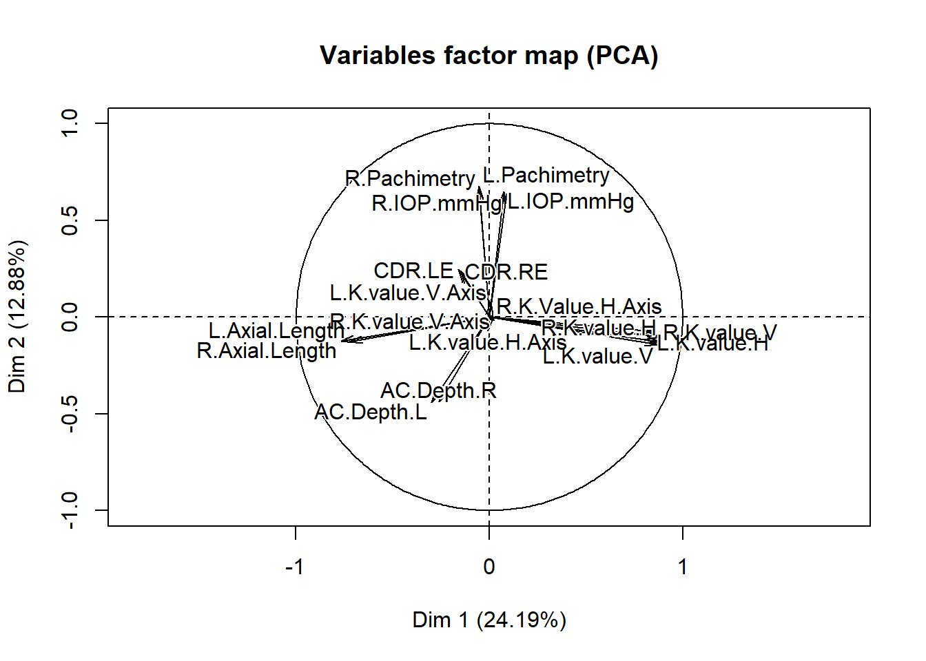
## 6         20    0.6    0.6

5. Perform PCA on the imputed data set and plot uncertainties

res.pca = PCA(res.comp$completeObs)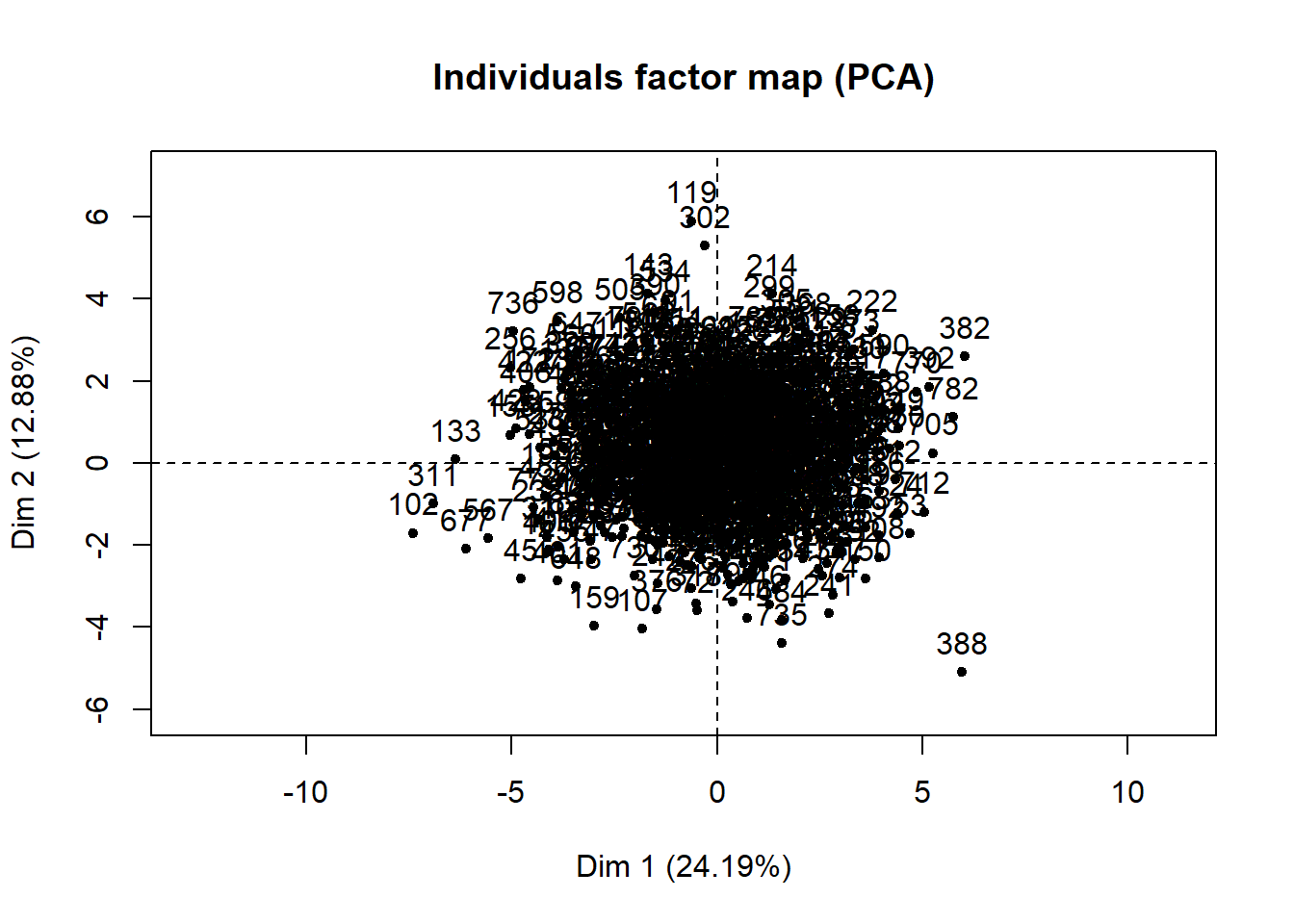

6. Perform multiple imputations

“res.comp = MIPCA(quant.data.adults, ncp = nb$ncp, nboot = 1000)”

Discussion

The single imputation has produced a complete dataset. It is difficult to interpret the individuals factor map in detail because there are a large number of individuals in the study, and each dot represents an individual. If any of the participants had a signifiant amount of data missing, a circle around the dot would be present signifying the uncertainty of the imputed values. The larger the area of the circle, the higher the uncertainty. However, there does not appear to be any that are clearly visible in this plot, which suggests that the imputed values for each individual fits well. It also possible that any circles that are present are not visible because of the dense cluster of dots in the plot. The variables factor map shows the uncertainty of the imputed values for each variable.

https://cran.r-project.org/web/packages/missMDA/missMDA.pdf http://factominer.free.fr/missMDA/PCA.html http://www.statpower.net/Content/312/R%20Stuff/PCA.html

The results of this PCA imputation does not show the variation for each individual or variable as it was only performed once. Variation, or uncertainty, of the imputed values can be determined by performing multiple imputations.