| tags: [ Data Cleaning Genomic Data Linux PLINK ] categories: [Coding Experiments ]
Generating stats for merged data and extracting data for NIES
Introduction
Now that the merge has been successful and there should no longer be duplicated individuals, general stats need to be performed on the merged data set. Subsequently, the final step to this data prep and cleaning is to extract data for the NIES individuals only.
Methods and Results
Note: Most processes up until the merge from the previous entry was performed on taurus. I transferred filtered_merge to local directory. These stat tests will be performed locally. ###1. Generate allele freq stats
plink --bfile plink_output/filtered_merge --freq --out plink_output/merge_allele_freq2. Load allele freq file
merged_allele_freq <- read.table('C:/Users/Martha/Documents/Honours/Project/honours.project/Data/plink_output/merged_allele_freq.frq', header = T)

head(merged_allele_freq)
## CHR SNP A1 A2 MAF NCHROBS
## 1 1 rs62637813 C G 0.125000 104
## 2 1 rs146477069 G A 0.009804 102
## 3 1 rs141149254 A G 0.031250 64
## 4 1 rs2462492 T C 0.425900 54
## 5 1 rs143174675 G T 0.009091 110
## 6 1 rs3091274 C A 0.000000 1103. Generate histogram for allele freq distributions
hist(merged_allele_freq$MAF, main = "Allele Frequency Distributions of Merged Data", xlab = "Minor Allele Frequency", xlim = c(0.0, 0.5), col = "plum2")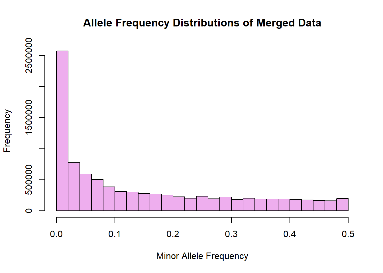
4. Generate missingness statistics
plink1.9 --bfile plink_output/filtered_merge --missing --out plink_output/merged_missingmerged_missing_snp <- read.table('C:/Users/Martha/Documents/Honours/Project/honours.project/Data/plink_output/merged_missing.lmiss', header = T)
head(merged_missing_snp)## CHR SNP N_MISS N_GENO F_MISS
## 1 1 rs62637813 64 520 0.12310
## 2 1 rs146477069 115 520 0.22120
## 3 1 rs141149254 264 520 0.50770
## 4 1 rs2462492 295 520 0.56730
## 5 1 rs143174675 34 520 0.06538
## 6 1 rs3091274 24 520 0.04615merged_missing_indiv <- read.table('C:/Users/Martha/Documents/Honours/Project/honours.project/Data/plink_output/merged_missing.imiss', header = T)
head(merged_missing_indiv)## FID IID MISS_PHENO N_MISS N_GENO F_MISS
## 1 1 110050 Y 243446 9155053 0.02659
## 2 1 110110 Y 278192 9155053 0.03039
## 3 1 110130 Y 267987 9155053 0.02927
## 4 1 110150 Y 250349 9155053 0.02735
## 5 1 110160 Y 235054 9155053 0.02567
## 6 1 110320 Y 277136 9155053 0.030275. Generate hardy-weinberg statistics
plink1.9 --bfile plink_output/filtered_merge --hardy --out plink_output/merged_hardy#merged_hardy <- read.table('C:/Users/Martha/Documents/Honours/Project/honours.project/Data/plink_output/merged_hardy.hwe', header = T)
#head(merged_hardy)6. Filter out variants based on HWE p-value
plink1.9 --bfile plink_output/filtered_merge --hwe 1.8e-7 --make-bed --out plink_output/merged_hwe_filterNote: unlike previous attempts at generating stats before merging, I did not use a HWE p-val filter before merging this data set. Note: this creates a new file set
Output: - 1897 variants were excluded based on hwe p-val - 9,153,156 variants remain - warning: hwe observation counts vary by more than 10%
7. Check allele freq stats after filtering
plink1.9 --bfile plink_output/merged_hwe_filter --freq --out plink_output/merge_hwefilter_freq8. Load allele freq file
merged_hwefilter_freq <- read.table('C:/Users/Martha/Documents/Honours/Project/honours.project/Data/plink_output/merge_hwefilter_freq.frq', header = T)9. Generate histogram of allele freq distributions
hist(merged_hwefilter_freq$MAF, main = "Allele Frequency Distributions of Merged Data after HWE filtering", xlab = "Minor Allele Frequency", xlim = c(0.0, 0.5), col = "peachpuff")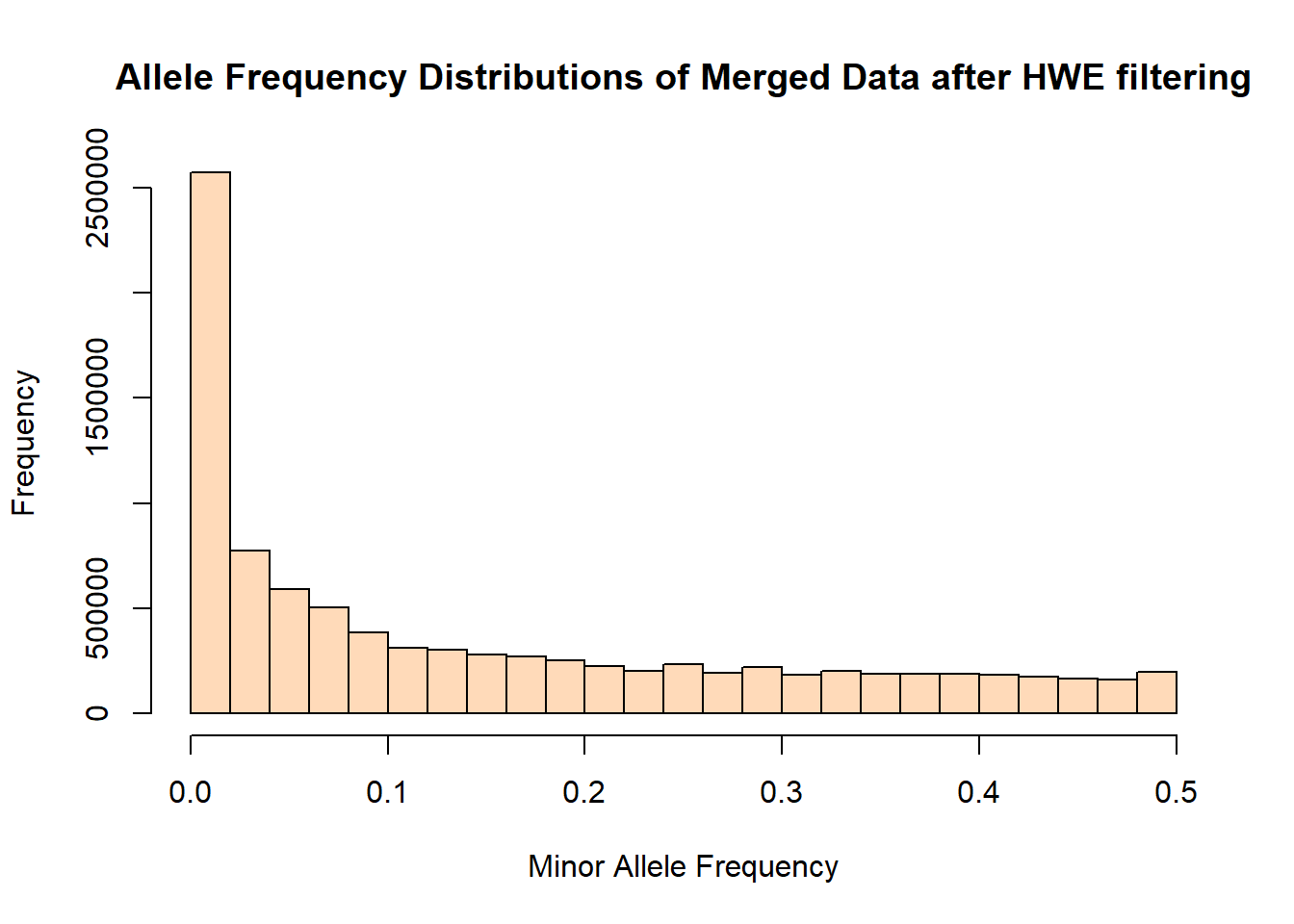
10. Load spreadsheet with NI study participants
ni_ped_uuid <- read.csv('C:/Users/Martha/Documents/Honours/Project/honours.project/Data/NI_UUID_Ped_20180718.csv', header = T)

head(ni_ped_uuid)
## UUID Ped_ID LAB_ID PID SID NIES KCCGID Gender DOB IN_2000
## 1 110020 NA 1002 <NA> <NA> <NA> <NA> Female 5/16/1929 1
## 2 110030 NA 1003 <NA> <NA> <NA> <NA> Female 5/23/1928 1
## 3 110040 3676 1004 <NA> <NA> <NA> <NA> Female 2/08/1959 1
## 4 110050 765 1005 <NA> <NA> <NA> <NA> Male 11/07/1954 1
## 5 110080 NA 1008 <NA> <NA> <NA> <NA> Female 10/07/1933 1
## 6 110090 NA 1009 <NA> <NA> <NA> <NA> Female 10/08/1968 1
## AGE_2000NIHS IN_2010 AGE_2010NIHS IN_NIES AGE_NIES RECOLLECT COREPED_1
## 1 71 0 80 0 79 0 0
## 2 72 0 81 0 80 0 0
## 3 41 0 50 0 49 0 0
## 4 46 0 55 0 54 0 1
## 5 67 0 76 0 75 0 0
## 6 32 0 41 0 40 0 0
## COREPED_2 Miles_core DNA_NIHS X2000NIHS_GWAS X2010NIHS_GWAS GWAS_NIHS
## 1 0 0 1 0 0 0
## 2 0 0 1 0 0 0
## 3 0 0 1 0 0 0
## 4 1 1 1 1 0 1
## 5 0 0 1 0 0 0
## 6 0 0 1 0 0 0
## DNA_NIES GWAS_NIES Total_GWAS NI_exprs WGS_data DNA_TOTAL
## 1 0 0 0 0 0 1
## 2 0 0 0 0 0 1
## 3 0 0 0 0 0 1
## 4 0 0 1 0 0 1
## 5 0 0 0 0 0 1
## 6 0 0 0 0 0 1
## Relation.to.NIHS.Pedigree..n.6379. patID matID Ped_Gender isParent
## 1 <NA> NA NA <NA> NA
## 2 <NA> NA NA <NA> NA
## 3 <NA> NA NA <NA> NA
## 4 <NA> 764 762 Male FALSE
## 5 <NA> NA NA <NA> NA
## 6 <NA> NA NA <NA> NA11. Isolate all NIES individuals using “NIES” column, and all NIES indivs with sequencing data using “GWAS_NIES” column
gwas_niesID <- read.csv('C:/Users/Martha/Documents/Honours/Project/honours.project/Data/gwas_niesID.csv', header = F)

head(gwas_niesID)
## V1
## 1 312481
## 2 311020
## 3 255711
## 4 321130
## 5 232110
## 6 253810There are 363 NIES individuals that may have sequencing data identified from the spreadsheet. This list was also converted to .txt to be compatible with PLINK.
12. Extract data in PLINK
plink1.9 --bfile plink_output/merged_hwe_filter --keep gwas_niesID.txt --make-bed --out merged_niesThis extracted data for only 361 individuals, which is 2 less than expected. I suspect it may be because of differing paternal and maternal IDs. Therefore, I changed all maternal and paternal IDs in “merged_hwe_filter.fam” to 0s but this did not resolve the issue. PLINK is still only extracting data for 361 individuals (9,153,156 variants; total genotyping rate = 91.68%)
The file sets created in this step will be used for all subsequent analysis.
13. Check allele frequencies of this final data set
plink1.9 --bfile merged_nies --freq --out plink_output/merged_nies_allele_freq14. Load allele freq file
merged_nies_allele_freq <- read.table('C:/Users/Martha/Documents/Honours/Project/honours.project/Data/plink_output/merged_nies_allele_freq.frq', header = T)

head(merged_nies_allele_freq)
## CHR SNP A1 A2 MAF NCHROBS
## 1 1 rs62637813 C G 0.014330 628
## 2 1 rs146477069 G A 0.003497 572
## 3 1 rs141149254 A G 0.063580 346
## 4 1 rs2462492 T C 0.155400 296
## 5 1 rs143174675 G T 0.002994 668
## 6 1 rs3091274 C A 0.000000 69015. Generate histogram for allele frequency distributions
hist(merged_nies_allele_freq$MAF, main = "Allele Frequency Distributions of NIES Data", xlab = "Minor Allele Frequency", xlim = c(0.0, 0.5), col = "lightskyblue1")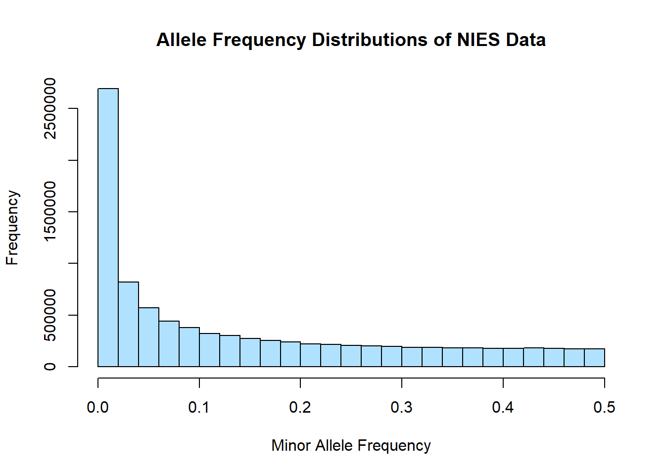
16. Check missingness rates
plink1.9 --bfile merged_nies --missing --out plink_output/merged_nies_missingmerged_nies_imissing <- read.table('C:/Users/Martha/Documents/Honours/Project/honours.project/Data/plink_output/merged_nies_missing.imiss', header = T)
head(merged_nies_imissing)## FID IID MISS_PHENO N_MISS N_GENO F_MISS
## 1 1 110150 Y 250197 9153156 0.02733
## 2 1 110160 Y 234913 9153156 0.02566
## 3 1 110500 Y 320553 9153156 0.03502
## 4 1 110650 Y 284393 9153156 0.03107
## 5 1 110820 Y 253220 9153156 0.02766
## 6 1 111280 Y 2841898 9153156 0.31050merged_nies_lmissing <- read.table('C:/Users/Martha/Documents/Honours/Project/honours.project/Data/plink_output/merged_nies_missing.lmiss', header = T)
head(merged_nies_lmissing)## CHR SNP N_MISS N_GENO F_MISS
## 1 1 rs62637813 47 361 0.13020
## 2 1 rs146477069 75 361 0.20780
## 3 1 rs141149254 188 361 0.52080
## 4 1 rs2462492 213 361 0.59000
## 5 1 rs143174675 27 361 0.07479
## 6 1 rs3091274 16 361 0.0443217. The current data set should be filtered for missingness rates.
PLINK’s default parameters excludes individuals with >10% missing genotypes, and SNPs with >10% missing calls. According to literature, typical QC excludes individuals with >2-7% missing genotypes, and SNPs with >1-5% mising calls. (https://www.ncbi.nlm.nih.gov/pmc/articles/PMC3061487/) (https://www.ncbi.nlm.nih.gov/pmc/articles/PMC3025522/)
plink1.9 --bfile merged_nies --mind 0.1 --geno 0.05 --make-bed --out merged_nies_miss_filterThis filters out individuals with >10% missing genotypes and SNPs with >5% missing call rates. By doing so, 73 individuals and 1,357,838 variants were filtered out. The new data set contains: 288 individuals and 7,795,318 variants, with a total genotpying rate of 97.10% (this genotyping rate has increased from 91.68%).
This filtering step excluded more individuals and variants than I expected. The exlcuded individuals had missing genotyping rates ranging from 19 - 31%. However, due to the modest number of samples in this study, we are reluctant to exclude any individuals and will therefore not be using a filter for missing genotypes per sample.
18. Apply genotyping rate filter for SNPs.
plink1.9 --bfile merged_nies --geno 0.1 --make-bed --out merged_nies_miss_filterThis filters out 3,465,839 variants. The final data set includes 361 individuals and 5,687,317 variants with a total genotyping rate of 91.68%.
19. Check allele frequencies for this filtered data set
plink1.9 --bfile merged_nies_miss_filter --freq --out plink_output/nies_geno0.1_allele_freqOutput: - 361 individuals - 5,687,317 variants - total genotyping rate = 95.78%
20. Load allele frequency file
nies_geno0.1_freq <- read.table('C:/Users/Martha/Documents/Honours/Project/honours.project/Data/plink_output/nies_geno0.1_allele_freq.frq', header = T)

head(nies_geno0.1_freq)
## CHR SNP A1 A2 MAF NCHROBS
## 1 1 rs143174675 G T 0.002994 668
## 2 1 rs3091274 C A 0.000000 690
## 3 1 rs183209871 A G 0.002801 714
## 4 1 rs4117992 T C 0.000000 716
## 5 1 rs79114531 C A 0.000000 716
## 6 1 rs2808353 G A 0.000000 70021. Generate histogram for allele frequency distribution
hist(nies_geno0.1_freq$MAF, main = "Allele Frequency Distributions of NIES Data Post-Geno Filtering", xlab = "Minor Allele Frequency", xlim = c(0.0, 0.5), col = "salmon1")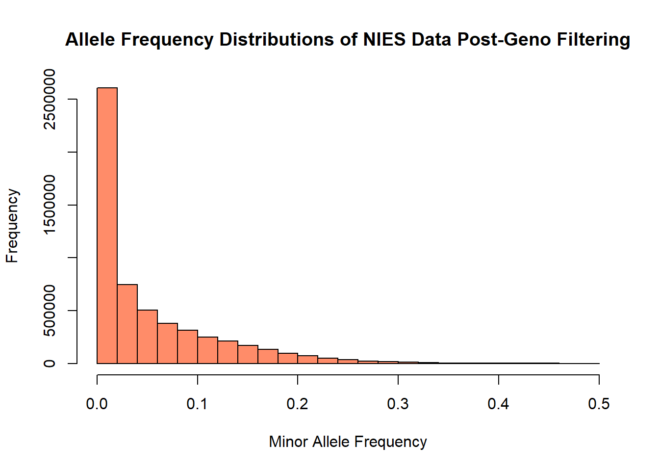
The allele frequency distribution of this filtered data set appears to retain roughly the same number of rare variants (MAR < 0.05). However, there is a noticeable change