| tags: [ Gaston Genomic Data Heritability ] categories: [Coding Experiments ]
Including principal components for estimating heritability
Introduction
Recent studies suggest that hidden population stratification can singificantly inflate heritability estimates. It is therefore imperative that population structure is accounted for when estimating heritability by including principal components in the linear mixed model. Typically, 10 to 20 principal components are used for this correction in outbred populations, but these numbers have no theoretical basis. A paper by Dandine-Roulland et al. (2016) has shown that heritability estimates are significantly affected with the inclusion of the first principal component, but not of any more (https://www.ncbi.nlm.nih.gov/pmc/articles/PMC4879529/).
We expect that the same effect will be observed with my data and therefore, I will compare heritability estimates produced with 0, 1, 2, or 3 principal components included in the linear mixed model.
Methods and Results
In the last exercise, I did not consider the sigma-squared and tau values, which are used to calculate heritability estimates.
tau = estimated genetic variance
sigma2 = estimated residual variance
tau + sigma2 = total variance
Therefore, tau/(tau + sigma2) = estimated heritability
For this exercise, I will calculate the heritability estimates for individual variables which have known/previously calculated heritability estimates (e.g. IOP, CDR, AC depth, etc.) using tau and sigma2 values. I will also test for the inclusion of 0, 1, 2, or 3 principal components in the linear mixed model. The aim for this is to determine a suitable number of principal components that will adequately correct for population stratification so that the heritability estimate obtained is not inflated. Once this is determined, the no. of PCs will be included in the calculation of heritability estimates for the rest of the phenotypic variables, and then for the phenotypic principal components. Confidence intervals will then be calculated to determine which variables are significantly heritable.
1. Generate phenotypic data
imputed_phen_data <- read.csv('C:/Users/Martha/Documents/Honours/Project/honours.project/imputed_phenotypic_data_uvaf.csv', header = T)
merged_nies_fam <- read.table('C:/Users/Martha/Documents/Honours/Project/honours.project/Data/merged_nies_filtered.fam', header = F)
geno_data_uuid <- merged_nies_fam$V2
nies_pheno <- imputed_phen_data[imputed_phen_data$UUID %in% c(geno_data_uuid), ]
merged_nies_fam_210818 <- read.table('C:/Users/Martha/Documents/Honours/Project/honours.project/Data/merged_nies/merged_nies_geno_210818.fam', header = F)
geno_data_uuid2 <- merged_nies_fam_210818$V2
nies_pheno_210818 <- nies_pheno[nies_pheno$UUID %in% c(geno_data_uuid2), ] #final phenotypic data set
2. Load genomic data
require(gaston)## Loading required package: gaston## Loading required package: Rcpp## Loading required package: RcppParallel##
## Attaching package: 'RcppParallel'## The following object is masked from 'package:Rcpp':
##
## LdFlags## Gaston set number of threads to 2. Use setThreadOptions() to modify this.##
## Attaching package: 'gaston'## The following object is masked from 'package:stats':
##
## sigma## The following objects are masked from 'package:base':
##
## cbind, rbindmerged_nies_210818 <- read.bed.matrix("C:/Users/Martha/Documents/Honours/Project/honours.project/Data/merged_nies/merged_nies_geno_210818.bed")## Reading C:/Users/Martha/Documents/Honours/Project/honours.project/Data/merged_nies/merged_nies_geno_210818.fam
## Reading C:/Users/Martha/Documents/Honours/Project/honours.project/Data/merged_nies/merged_nies_geno_210818.bim
## Reading C:/Users/Martha/Documents/Honours/Project/honours.project/Data/merged_nies/merged_nies_geno_210818.bed
## ped stats and snps stats have been set.
## 'p' has been set.
## 'mu' and 'sigma' have been set.3. Generate GRM and calculate eigen decomposition
merged_nies_GRM <- GRM(merged_nies_210818)

merged_nies_eiK <- eigen(merged_nies_GRM)

merged_nies_eiK$values[ merged_nies_eiK$values < 0] <- 0
4. Calculate heritability of anterior chamber depth
#for Right AC depth values
#with 0 PCs
fit.R.acd0 <- lmm.diago(nies_pheno_210818$R.AC.Depth, eigenK = merged_nies_eiK)
## Optimization in interval [0, 1]
## Optimizing with p = 0
## [Iteration 1] Current point = 0 df = 27.2665
## [Iteration 2] Current point = 0.18723 df = 8.27687
## [Iteration 3] Current point = 0.296964 df = 0.659801
## [Iteration 4] Current point = 0.307044 df = 0.00182903
## [Iteration 5] Current point = 0.307072 df = 1.20226e-008h2.R.acd0 <- fit.R.acd0$tau / (fit.R.acd0$tau + fit.R.acd0$sigma2)
h2.R.acd0## [1] 0.3070724#with 1PC
fit.R.acd1 <- lmm.diago(nies_pheno_210818$R.AC.Depth, eigenK = merged_nies_eiK, p = 1)## Optimization in interval [0, 1]
## Optimizing with p = 1
## [Iteration 1] Current point = 0 df = 29.4602
## [Iteration 2] Current point = 0.190022 df = 9.32351
## [Iteration 3] Current point = 0.310278 df = 0.821886
## [Iteration 4] Current point = 0.322658 df = 0.00237211
## [Iteration 5] Current point = 0.322694 df = 1.55365e-008h2.R.acd1<- fit.R.acd1$tau / (fit.R.acd1$tau + fit.R.acd1$sigma2)
h2.R.acd1## [1] 0.3226943#with 2PCs
fit.R.acd2 <- lmm.diago(nies_pheno_210818$R.AC.Depth, eigenK = merged_nies_eiK, p = 2)## Optimization in interval [0, 1]
## Optimizing with p = 2
## [Iteration 1] Current point = 0 df = 25.019
## [Iteration 2] Current point = 0.208385 df = 6.76504
## [Iteration 3] Current point = 0.307491 df = 0.337584
## [Iteration 4] Current point = 0.312871 df = 0.000239402h2.R.acd2<- fit.R.acd2$tau / (fit.R.acd2$tau + fit.R.acd2$sigma2)
h2.R.acd2## [1] 0.3128744#with 3 PCs
fit.R.acd3 <- lmm.diago(nies_pheno_210818$R.AC.Depth, eigenK = merged_nies_eiK, p = 3)## Optimization in interval [0, 1]
## Optimizing with p = 3
## [Iteration 1] Current point = 0 df = 25.1127
## [Iteration 2] Current point = 0.215881 df = 6.6785
## [Iteration 3] Current point = 0.315489 df = 0.296111
## [Iteration 4] Current point = 0.320238 df = 0.000109947h2.R.acd3<- fit.R.acd3$tau / (fit.R.acd3$tau + fit.R.acd3$sigma2)
h2.R.acd3## [1] 0.3202402#for Left AC depth values
#with 0 PCs
fit.L.acd0 <- lmm.diago(nies_pheno_210818$L.AC.Depth, eigenK = merged_nies_eiK)## Optimization in interval [0, 1]
## Optimizing with p = 0
## [Iteration 1] Current point = 0 df = 25.4208
## [Iteration 2] Current point = 0.180651 df = 7.2106
## [Iteration 3] Current point = 0.274918 df = 0.536193
## [Iteration 4] Current point = 0.282972 df = 0.00194078
## [Iteration 5] Current point = 0.283001 df = 2.39764e-008h2.L.acd0<- fit.L.acd0$tau / (fit.L.acd0$tau + fit.L.acd0$sigma2)
h2.L.acd0## [1] 0.2830011#with 1 PC
fit.L.acd1 <- lmm.diago(nies_pheno_210818$L.AC.Depth, eigenK = merged_nies_eiK, p = 1)## Optimization in interval [0, 1]
## Optimizing with p = 1
## [Iteration 1] Current point = 0 df = 27.4071
## [Iteration 2] Current point = 0.184896 df = 8.09619
## [Iteration 3] Current point = 0.28852 df = 0.659931
## [Iteration 4] Current point = 0.298344 df = 0.0026655
## [Iteration 5] Current point = 0.298384 df = 4.00844e-008h2.L.acd1<- fit.L.acd1$tau / (fit.L.acd1$tau + fit.L.acd1$sigma2)
h2.L.acd1## [1] 0.2983835#with 2 PCs
fit.L.acd2 <- lmm.diago(nies_pheno_210818$L.AC.Depth, eigenK = merged_nies_eiK, p = 2)## Optimization in interval [0, 1]
## Optimizing with p = 2
## [Iteration 1] Current point = 0 df = 24.4286
## [Iteration 2] Current point = 0.198858 df = 6.34809
## [Iteration 3] Current point = 0.288122 df = 0.349883
## [Iteration 4] Current point = 0.293561 df = 0.000614758
## [Iteration 5] Current point = 0.293571 df = 1.79782e-009h2.L.acd2<- fit.L.acd2$tau / (fit.L.acd2$tau + fit.L.acd2$sigma2)
h2.L.acd2## [1] 0.2935709#with 3 PCs
fit.L.acd3 <- lmm.diago(nies_pheno_210818$L.AC.Depth, eigenK = merged_nies_eiK, p = 3)## Optimization in interval [0, 1]
## Optimizing with p = 3
## [Iteration 1] Current point = 0 df = 24.7661
## [Iteration 2] Current point = 0.205596 df = 6.3916
## [Iteration 3] Current point = 0.296709 df = 0.332728
## [Iteration 4] Current point = 0.301918 df = 0.000477792
## [Iteration 5] Current point = 0.301926 df = 9.26967e-010h2.L.acd3<- fit.L.acd3$tau / (fit.L.acd3$tau + fit.L.acd3$sigma2)
h2.L.acd3## [1] 0.3019255Current heritability estimate for ACD in NI from previous studies = 0.4
5. Calculate heritability estimates for IOP
#for R IOP
#with 0 PCs
fit.R.iop0 <- lmm.diago(nies_pheno_210818$R.IOP.mmHg, eigenK = merged_nies_eiK)## Optimization in interval [0, 1]
## Optimizing with p = 0
## [Iteration 1] Current point = 0 df = 19.0563
## [Iteration 2] Current point = 0.147446 df = 6.12048
## [Iteration 3] Current point = 0.24176 df = 0.503822
## [Iteration 4] Current point = 0.250745 df = 0.00152377
## [Iteration 5] Current point = 0.250772 df = 1.21091e-008fit.R.iop0$tau / (fit.R.iop0$tau + fit.R.iop0$sigma2)## [1] 0.2507722#with 1 PC
fit.R.iop1 <- lmm.diago(nies_pheno_210818$R.IOP.mmHg, eigenK = merged_nies_eiK, p = 1)## Optimization in interval [0, 1]
## Optimizing with p = 1
## [Iteration 1] Current point = 0 df = 15.4492
## [Iteration 2] Current point = 0.179204 df = 3.60924
## [Iteration 3] Current point = 0.245273 df = 0.0926403
## [Iteration 4] Current point = 0.247042 df = 1.71739e-005fit.R.iop1$tau / (fit.R.iop1$tau + fit.R.iop1$sigma2)## [1] 0.2470424#with 2 PCs
fit.R.iop2 <- lmm.diago(nies_pheno_210818$R.IOP.mmHg, eigenK = merged_nies_eiK, p = 2)## Optimization in interval [0, 1]
## Optimizing with p = 2
## [Iteration 1] Current point = 0 df = 17.157
## [Iteration 2] Current point = 0.18723 df = 4.28128
## [Iteration 3] Current point = 0.263656 df = 0.122049
## [Iteration 4] Current point = 0.265935 df = 1.29855e-005fit.R.iop2$tau / (fit.R.iop2$tau + fit.R.iop2$sigma2)## [1] 0.2659357#with 3 PCs
fit.R.iop3 <- lmm.diago(nies_pheno_210818$R.IOP.mmHg, eigenK = merged_nies_eiK, p = 3)## Optimization in interval [0, 1]
## Optimizing with p = 3
## [Iteration 1] Current point = 0 df = 17.2637
## [Iteration 2] Current point = 0.196526 df = 4.18823
## [Iteration 3] Current point = 0.272802 df = 0.0907274
## [Iteration 4] Current point = 0.274508 df = -4.17165e-006fit.R.iop3$tau / (fit.R.iop3$tau + fit.R.iop3$sigma2)## [1] 0.2745082#for L IOP
#with 0 PCs
fit.L.iop0 <- lmm.diago(nies_pheno_210818$L.IOP.mmHg, eigenK = merged_nies_eiK)## Optimization in interval [0, 1]
## Optimizing with p = 0
## [Iteration 1] Current point = 0 df = 19.565
## [Iteration 2] Current point = 0.131325 df = 5.87129
## [Iteration 3] Current point = 0.206538 df = 0.500194
## [Iteration 4] Current point = 0.214074 df = 0.00268863
## [Iteration 5] Current point = 0.214115 df = 7.4301e-008fit.L.iop0$tau / (fit.L.iop0$tau + fit.L.iop0$sigma2)## [1] 0.2141154#with 1 PC
fit.L.iop1 <- lmm.diago(nies_pheno_210818$L.IOP.mmHg, eigenK = merged_nies_eiK, p = 1)## Optimization in interval [0, 1]
## Optimizing with p = 1
## [Iteration 1] Current point = 0 df = 14.8268
## [Iteration 2] Current point = 0.154697 df = 3.01726
## [Iteration 3] Current point = 0.201948 df = 0.0893711
## [Iteration 4] Current point = 0.203428 df = 5.82493e-005fit.L.iop1$tau / (fit.L.iop1$tau + fit.L.iop1$sigma2)## [1] 0.2034288#with 2 PCs
fit.L.iop2 <- lmm.diago(nies_pheno_210818$L.IOP.mmHg, eigenK = merged_nies_eiK, p = 2)## Optimization in interval [0, 1]
## Optimizing with p = 2
## [Iteration 1] Current point = 0 df = 15.7871
## [Iteration 2] Current point = 0.164015 df = 3.26658
## [Iteration 3] Current point = 0.21526 df = 0.0952811
## [Iteration 4] Current point = 0.216838 df = 5.61709e-005fit.L.iop2$tau / (fit.L.iop2$tau + fit.L.iop2$sigma2)## [1] 0.2168385#with 3 PCs
fit.L.iop3 <- lmm.diago(nies_pheno_210818$L.IOP.mmHg, eigenK = merged_nies_eiK, p = 3)## Optimization in interval [0, 1]
## Optimizing with p = 3
## [Iteration 1] Current point = 0 df = 17.2376
## [Iteration 2] Current point = 0.172355 df = 3.77221
## [Iteration 3] Current point = 0.230781 df = 0.119681
## [Iteration 4] Current point = 0.232745 df = 7.56419e-005fit.L.iop3$tau / (fit.L.iop3$tau + fit.L.iop3$sigma2)## [1] 0.2327464#with 10 PCs
fit.L.iop10 <- lmm.diago(nies_pheno_210818$L.IOP.mmHg, eigenK = merged_nies_eiK, p = 10)## Optimization in interval [0, 1]
## Optimizing with p = 10
## [Iteration 1] Current point = 0 df = 12.1457
## [Iteration 2] Current point = 0.191892 df = 1.5919
## [Iteration 3] Current point = 0.223357 df = 0.00388723
## [Iteration 4] Current point = 0.223434 df = -3.95619e-009fit.L.iop10$tau / (fit.L.iop10$tau + fit.L.iop10$sigma2)## [1] 0.2234345Current heritability estimate for IOP in NI from previous studies = 0.35
The above calculations indicate that the estimates fluctuate somewhat (+/- 2%) with the inclusion of up to 3 PCs. In the study mentioned above (https://www.ncbi.nlm.nih.gov/pmc/articles/PMC4879529/) the inclusion of 1 PC clearly decreases the estimates by ~7% and adding more PCs does not change this. Thus, it seems as if adding PCs to the model for my data does not significantly change the heritability estimates. This may be because the samples in this study is part of a single core pedigree (therefore no expected hidden population stratification?), whereas the study by Dandine-Roulland et al. (2016) is performed on an outbred population and involves 5700+ individuals.
Additionally, my estimates are ~10% less than the previous estimates for the same variables in the NI population. However, this is most likely due to the difference in sample sizes, having more SNVs, and a more robust estimation method in this study.
Based on these observations, there is no reason to include more than 2 PCs when estimating heritability of the other variables.
6. Test lmm.diago.likelihood function to find confidence intervals for the heritability estimates
#for ACD
lik.R.acd <- lmm.diago.likelihood(h2 = h2.R.acd2, Y = nies_pheno_210818$R.AC.Depth, eigenK = merged_nies_eiK, p=2)
lik.R.acd$likelihood## [1] 144.7306This function gives me a likelihood value but I don’t understand the significance of it. I need to know the p-value of the heritability estimate to determine the statistical significance of the estimate. After reading the documentation for gaston and the lmm.diago/lmm.diago.likelihood functions, I don’t believe that there is any way to obtain the p-value using these functions.
7. Plot likelihood to check heritability estimate
H2 <- seq(0,1,length=51)
Lik <- lmm.diago.likelihood(h2 = H2, Y=nies_pheno_210818$R.AC.Depth, eigenK = merged_nies_eiK, p=2)
plot(H2, exp(Lik$likelihood), type = "l", yaxt = "n",ylab = "likelihood", main = "Right ACD")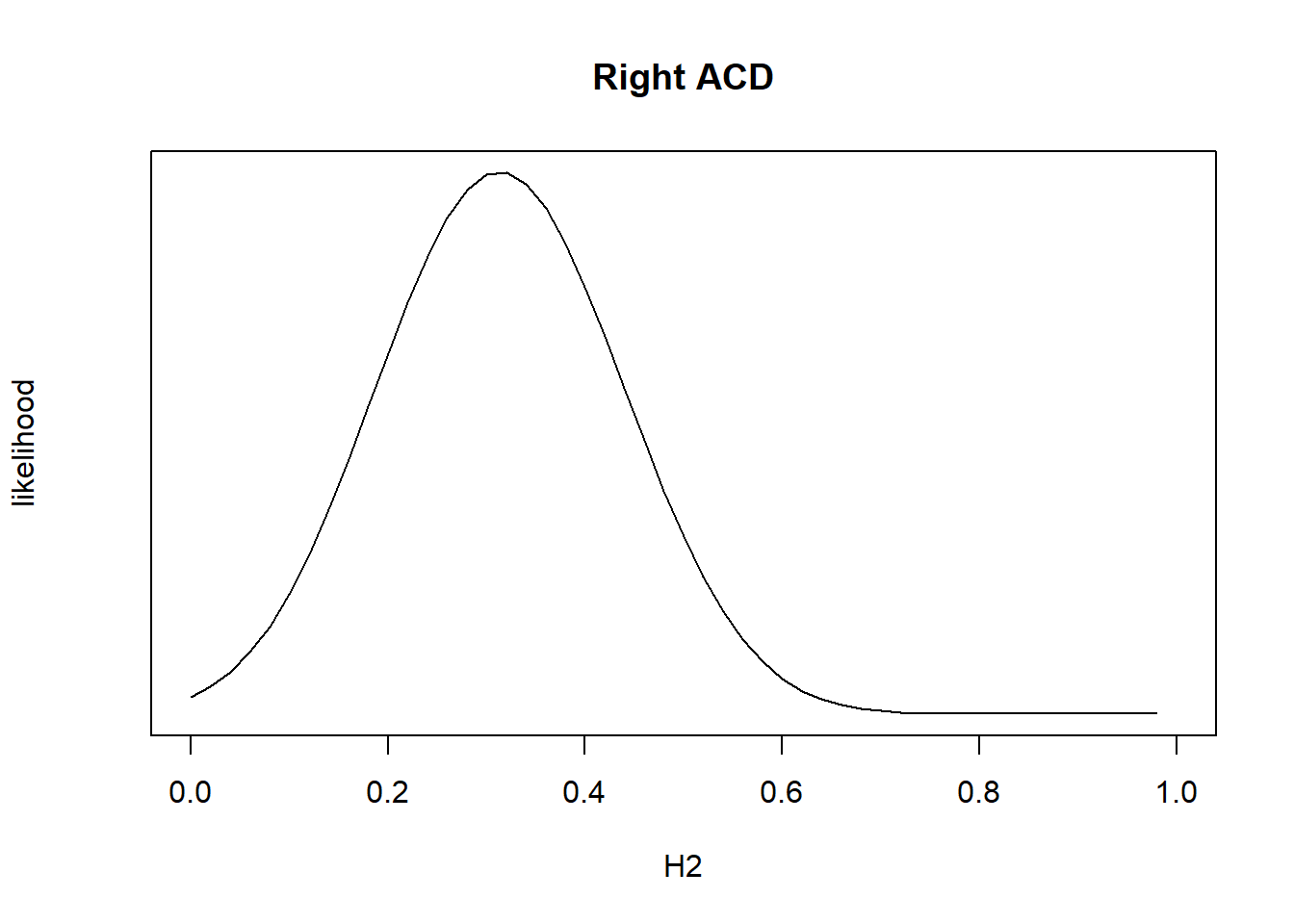
7. Calculate heritability estimates for all of the individual phenotypic variables
require(magicfor)## Loading required package: magicformagic_for(print, silent = T)
for (i in 2:ncol(nies_pheno_210818)){
variable1 <- colnames(nies_pheno_210818[i])
fit <- lmm.diago(nies_pheno_210818[,i], eigenK = merged_nies_eiK, p=2)
h2 <- fit$tau/(fit$tau + fit$sigma2)
lik <- lmm.diago.likelihood(h2 = h2, Y = nies_pheno_210818[,i], eigenK = merged_nies_eiK, p=2)
print(Variable = variable1, h2, likelihood = lik$likelihood)
}## Optimization in interval [0, 1]
## Optimizing with p = 2
## [Iteration 1] Current point = 0 df = -7.11013
## [Iteration 1] maximum at min = 0
## Optimization in interval [0, 1]
## Optimizing with p = 2
## [Iteration 1] Current point = 0 df = -13.3561
## [Iteration 1] maximum at min = 0
## Optimization in interval [0, 1]
## Optimizing with p = 2
## [Iteration 1] Current point = 0 df = -8.19357
## [Iteration 1] maximum at min = 0
## Optimization in interval [0, 1]
## Optimizing with p = 2
## [Iteration 1] Current point = 0 df = 28.7103
## [Iteration 2] Current point = 0.599149 df = -3.46492
## [Iteration 3] Current point = 0.561391 df = -0.198617
## [Iteration 4] Current point = 0.558957 df = -0.000713875
## [Iteration 5] Current point = 0.558948 df = -9.27375e-009
## Optimization in interval [0, 1]
## Optimizing with p = 2
## [Iteration 1] Current point = 0 df = 3.78121
## [Iteration 2] Current point = 0.0614073 df = 0.309897
## [Iteration 3] Current point = 0.0673109 df = 0.00175775
## [Iteration 4] Current point = 0.0673448 df = 5.52169e-008
## Optimization in interval [0, 1]
## Optimizing with p = 2
## [Iteration 1] Current point = 0 df = -10.5435
## [Iteration 1] maximum at min = 0
## Optimization in interval [0, 1]
## Optimizing with p = 2
## [Iteration 1] Current point = 0 df = -4.78203
## [Iteration 1] maximum at min = 0
## Optimization in interval [0, 1]
## Optimizing with p = 2
## [Iteration 1] Current point = 0 df = 6.30518
## [Iteration 2] Current point = 0.0910141 df = 0.794675
## [Iteration 3] Current point = 0.105783 df = 0.011704
## [Iteration 4] Current point = 0.106007 df = 2.46312e-006
## Optimization in interval [0, 1]
## Optimizing with p = 2
## [Iteration 1] Current point = 0 df = 29.269
## [Iteration 2] Current point = 0.347647 df = 9.62902
## [Iteration 3] Current point = 0.542008 df = -1.62963
## [Iteration 4] Current point = 0.519432 df = -0.0548232
## [Iteration 5] Current point = 0.518619 df = -6.32935e-005
## Optimization in interval [0, 1]
## Optimizing with p = 2
## [Iteration 1] Current point = 0 df = -7.36338
## [Iteration 1] maximum at min = 0
## Optimization in interval [0, 1]
## Optimizing with p = 2
## [Iteration 1] Current point = 0 df = 34.8249
## [Iteration 2] Current point = 0.531217 df = 14.0813
## [Iteration 3] Current point = 0.879187 df = -27.5399
## [Iteration 4] Current point = 0.823716 df = -9.91648
## [Iteration 5] Current point = 0.775494 df = -2.20567
## [Iteration 6] Current point = 0.757915 df = -0.152536
## [Iteration 7] Current point = 0.756513 df = -0.000811872
## [Iteration 8] Current point = 0.756506 df = -2.31775e-008
## Optimization in interval [0, 1]
## Optimizing with p = 2
## [Iteration 1] Current point = 0 df = -11.3499
## [Iteration 1] maximum at min = 0
## Optimization in interval [0, 1]
## Optimizing with p = 2
## [Iteration 1] Current point = 0 df = 14.3799
## [Iteration 2] Current point = 0.263585 df = 1.54924
## [Iteration 3] Current point = 0.295381 df = -0.0212347
## [Iteration 4] Current point = 0.294957 df = -4.56719e-006
## Optimization in interval [0, 1]
## Optimizing with p = 2
## [Iteration 1] Current point = 0 df = -0.187161
## [Iteration 1] maximum at min = 0
## Optimization in interval [0, 1]
## Optimizing with p = 2
## [Iteration 1] Current point = 0 df = 29.0126
## [Iteration 2] Current point = 0.435271 df = 8.12837
## [Iteration 3] Current point = 0.613725 df = -1.21958
## [Iteration 4] Current point = 0.59433 df = -0.0309852
## [Iteration 5] Current point = 0.593811 df = -2.01423e-005
## Optimization in interval [0, 1]
## Optimizing with p = 2
## [Iteration 1] Current point = 0 df = -2.94506
## [Iteration 1] maximum at min = 0
## Optimization in interval [0, 1]
## Optimizing with p = 2
## [Iteration 1] Current point = 0 df = 36.5065
## [Iteration 2] Current point = 0.356508 df = 12.8279
## [Iteration 3] Current point = 0.610013 df = -0.571562
## [Iteration 4] Current point = 0.600536 df = -0.0047655
## [Iteration 5] Current point = 0.600456 df = -3.27571e-007
## Optimization in interval [0, 1]
## Optimizing with p = 2
## [Iteration 1] Current point = 0 df = 40.347
## [Iteration 2] Current point = 0.363064 df = 15.4634
## [Iteration 3] Current point = 0.677099 df = -0.587165
## [Iteration 4] Current point = 0.667423 df = -0.00565348
## [Iteration 5] Current point = 0.667328 df = -5.21474e-007
## Optimization in interval [0, 1]
## Optimizing with p = 2
## [Iteration 1] Current point = 0 df = 21.8958
## [Iteration 2] Current point = 0.254171 df = 5.84146
## [Iteration 3] Current point = 0.3687 df = 0.125045
## [Iteration 4] Current point = 0.37121 df = -5.02903e-005
## Optimization in interval [0, 1]
## Optimizing with p = 2
## [Iteration 1] Current point = 0 df = 20.5946
## [Iteration 2] Current point = 0.243888 df = 5.45003
## [Iteration 3] Current point = 0.351788 df = 0.10615
## [Iteration 4] Current point = 0.353935 df = -3.52901e-005
## Optimization in interval [0, 1]
## Optimizing with p = 2
## [Iteration 1] Current point = 0 df = 25.019
## [Iteration 2] Current point = 0.208385 df = 6.76504
## [Iteration 3] Current point = 0.307491 df = 0.337584
## [Iteration 4] Current point = 0.312871 df = 0.000239402
## Optimization in interval [0, 1]
## Optimizing with p = 2
## [Iteration 1] Current point = 0 df = 24.4286
## [Iteration 2] Current point = 0.198858 df = 6.34809
## [Iteration 3] Current point = 0.288122 df = 0.349883
## [Iteration 4] Current point = 0.293561 df = 0.000614758
## [Iteration 5] Current point = 0.293571 df = 1.79782e-009
## Optimization in interval [0, 1]
## Optimizing with p = 2
## [Iteration 1] Current point = 0 df = 17.157
## [Iteration 2] Current point = 0.18723 df = 4.28128
## [Iteration 3] Current point = 0.263656 df = 0.122049
## [Iteration 4] Current point = 0.265935 df = 1.29855e-005
## Optimization in interval [0, 1]
## Optimizing with p = 2
## [Iteration 1] Current point = 0 df = 15.7871
## [Iteration 2] Current point = 0.164015 df = 3.26658
## [Iteration 3] Current point = 0.21526 df = 0.0952811
## [Iteration 4] Current point = 0.216838 df = 5.61709e-005
## Optimization in interval [0, 1]
## Optimizing with p = 2
## [Iteration 1] Current point = 0 df = 33.0992
## [Iteration 2] Current point = 0.327339 df = 13.6128
## [Iteration 3] Current point = 0.632864 df = -2.41685
## [Iteration 4] Current point = 0.598798 df = -0.117288
## [Iteration 5] Current point = 0.596974 df = -0.000289291
## [Iteration 6] Current point = 0.596969 df = -1.76379e-009
## Optimization in interval [0, 1]
## Optimizing with p = 2
## [Iteration 1] Current point = 0 df = 30.6574
## [Iteration 2] Current point = 0.2758 df = 12.4104
## [Iteration 3] Current point = 0.5439 df = -0.185709
## [Iteration 4] Current point = 0.540475 df = -0.000632608
## [Iteration 5] Current point = 0.540463 df = -7.32253e-009
## Optimization in interval [0, 1]
## Optimizing with p = 2
## [Iteration 1] Current point = 0 df = 24.2256
## [Iteration 2] Current point = 0.303903 df = 7.32815
## [Iteration 3] Current point = 0.464196 df = -0.252431
## [Iteration 4] Current point = 0.459249 df = -0.000927276
## [Iteration 5] Current point = 0.459231 df = -1.23407e-008h2.results <-magic_result_as_dataframe(2:ncol(nies_pheno_210818))
h2.results## i Variable h2 likelihood
## 1 2 R.Logmar.VA 0.0000000 316.62416
## 2 3 L.Logmar.VA 0.0000000 321.24288
## 3 4 R.Sph..pre.dilate. 0.0000000 -264.02867
## 4 5 R.Cyl..pre.dilate. 0.5589481 -136.97940
## 5 6 R.Axis..pre.dilate. 0.0673448 -1552.59195
## 6 7 L.Sph..pre.dilate. 0.0000000 -291.56451
## 7 8 L.Cyl..pre.dilate. 0.0000000 -209.54878
## 8 9 L.Axis..pre.dilate. 0.1060066 -1563.90944
## 9 10 R.K.value.H 0.5186182 -304.08083
## 10 11 R.K.Value.H.Axis 0.0000000 -1563.96173
## 11 12 R.K.value.V 0.7565059 -322.36036
## 12 13 R.K.value.V.Axis 0.0000000 -1521.86874
## 13 14 L.K.value.H 0.2949570 -344.00925
## 14 15 L.K.value.H.Axis 0.0000000 -1572.85719
## 15 16 L.K.value.V 0.5938109 -316.15810
## 16 17 L.K.value.V.Axis 0.0000000 -1508.87061
## 17 18 R.Pachimetry 0.6004561 -1348.83239
## 18 19 L.Pachimetry 0.6673277 -1356.45538
## 19 20 R.Axial.Length 0.3712087 -95.00351
## 20 21 L.Axial.Length 0.3539338 -111.45304
## 21 22 R.AC.Depth 0.3128744 144.73059
## 22 23 L.AC.Depth 0.2935709 115.06771
## 23 24 R.IOP.mmHg 0.2659357 -542.55482
## 24 25 L.IOP.mmHg 0.2168385 -540.46397
## 25 26 R.CDR 0.5969690 384.16769
## 26 27 L.CDR 0.5404634 397.73078
## 27 28 totaluvafmm 0.4592306 -1298.94823Heritability estimates also need to be calculated for the 9 principal components identified in the first objective.
8. Load data from phenotypic principal components
pca_indiv <- read.csv('C:/Users/Martha/Documents/Honours/Project/honours.project/pca_indiv_results.csv', header = T)
coord <- c("UUID","coord.Dim.1", "coord.Dim.2", "coord.Dim.3", "coord.Dim.4", "coord.Dim.5", "coord.Dim.6", "coord.Dim.7",
           "coord.Dim.8", "coord.Dim.9")
pca_indiv_coord <- pca_indiv[coord]
pca_indiv_coord2 <- pca_indiv_coord[pca_indiv_coord$UUID %in% c(geno_data_uuid2), ]
write.csv(pca_indiv_coord2, 'C:/Users/Martha/Documents/Honours/Project/honours.project/Data/pheno_pca_coord.csv', row.names = F)9. Calculate heritability estimates for principal components
magic_for(print, silent = T)
for (i in 2:ncol(pca_indiv_coord2)){
  variable2 <- colnames(pca_indiv_coord2[i])
  fit2 <- lmm.diago(pca_indiv_coord2[,i], eigenK = merged_nies_eiK, p=2)
  h2 <- fit2$tau/(fit2$tau + fit2$sigma2)
  lik2 <- lmm.diago.likelihood(h2 = h2, Y = pca_indiv_coord2[,i], eigenK = merged_nies_eiK, p=2)
  print(Variable = variable2, h2, likelihood = lik2$likelihood)
}
## Optimization in interval [0, 1]
## Optimizing with p = 2
## [Iteration 1] Current point = 0 df = 32.1324
## [Iteration 2] Current point = 0.43118 df = 10.3438
## [Iteration 3] Current point = 0.655946 df = -2.42438
## [Iteration 4] Current point = 0.624108 df = -0.134976
## [Iteration 5] Current point = 0.622124 df = -0.000435264
## [Iteration 6] Current point = 0.622118 df = -4.53569e-009
## Optimization in interval [0, 1]
## Optimizing with p = 2
## [Iteration 1] Current point = 0 df = 9.679
## [Iteration 2] Current point = 0.181091 df = 1.51115
## [Iteration 3] Current point = 0.218667 df = 0.012992
## [Iteration 4] Current point = 0.218995 df = 4.54191e-007
## Optimization in interval [0, 1]
## Optimizing with p = 2
## [Iteration 1] Current point = 0 df = 19.5808
## [Iteration 2] Current point = 0.187983 df = 4.43599
## [Iteration 3] Current point = 0.252207 df = 0.0353046
## [Iteration 4] Current point = 0.252722 df = -2.47452e-006
## Optimization in interval [0, 1]
## Optimizing with p = 2
## [Iteration 1] Current point = 0 df = 32.0964
## [Iteration 2] Current point = 0.280623 df = 11.1789
## [Iteration 3] Current point = 0.478465 df = -0.0372614
## [Iteration 4] Current point = 0.477851 df = -1.52999e-005
## Optimization in interval [0, 1]
## Optimizing with p = 2
## [Iteration 1] Current point = 0 df = -3.11006
## [Iteration 1] maximum at min = 0
## Optimization in interval [0, 1]
## Optimizing with p = 2
## [Iteration 1] Current point = 0 df = 9.81468
## [Iteration 2] Current point = 0.116729 df = 1.35741
## [Iteration 3] Current point = 0.13781 df = 0.0182816
## [Iteration 4] Current point = 0.138102 df = 2.92277e-006
## Optimization in interval [0, 1]
## Optimizing with p = 2
## [Iteration 1] Current point = 0 df = 18.1204
## [Iteration 2] Current point = 0.212656 df = 3.86442
## [Iteration 3] Current point = 0.279803 df = 0.0417537
## [Iteration 4] Current point = 0.280539 df = -1.82371e-006
## Optimization in interval [0, 1]
## Optimizing with p = 2
## [Iteration 1] Current point = 0 df = 25.044
## [Iteration 2] Current point = 0.17053 df = 5.33242
## [Iteration 3] Current point = 0.225899 df = 0.153398
## [Iteration 4] Current point = 0.227578 df = 7.84673e-005
## Optimization in interval [0, 1]
## Optimizing with p = 2
## [Iteration 1] Current point = 0 df = -0.110252
## [Iteration 1] maximum at min = 0h2.pca.results <-magic_result_as_dataframe(2:ncol(pca_indiv_coord2))
h2.pca.results## i Variable h2 likelihood
## 1 2 coord.Dim.1 0.6221178 -397.0557
## 2 3 coord.Dim.2 0.2189946 -344.8495
## 3 4 coord.Dim.3 0.2527220 -381.9100
## 4 5 coord.Dim.4 0.4778504 -291.2495
## 5 6 coord.Dim.5 0.0000000 -299.9143
## 6 7 coord.Dim.6 0.1381016 -279.4047
## 7 8 coord.Dim.7 0.2805392 -198.2305
## 8 9 coord.Dim.8 0.2275784 -208.0908
## 9 10 coord.Dim.9 0.0000000 -187.1762