Introduction

After obtaining heritability estimates for all traits and principal components, I can prioritise the traits for GWAS. There are different methods for performing GWAS and analysing GWAS results in GCTA. In particular, I am interested in the MLMA method which is mixed linear model associations (https://www.ncbi.nlm.nih.gov/pubmed/24473328).

Methods and Results

1. Run GWAS-MLMA on R K-value V

./gcta64 --mlma --bfile merged_nies/merged_nies_geno_210818 --grm gcta_output/merged_nies_grm --pheno nies_pheno_020918.txt --mpheno 11 --out gcta_output/r_kval_mlma

r_kvalV_mlma <- read.table('C:/Users/Martha/Documents/Honours/Project/honours.project/Data/gcta_output/r_kval_mlma.mlma', header = TRUE)

head(r_kvalV_mlma)

##   Chr         SNP     bp A1 A2       Freq           b       se        p
## 1   1   rs2808353 590318  G  A 0.01449280 -0.06731680 0.534089 0.899700
## 2   1 rs138660747 778897  A  C 0.00434783 -0.16304800 1.113150 0.883547
## 3   1  rs10751453 783175  T  C 0.00000000         NaN      Inf      NaN
## 4   1   rs3131973 804046  A  G 0.00000000         NaN      Inf      NaN
## 5   1   rs3094315 817186  G  A 0.16666700 -0.14247400 0.191881 0.457777
## 6   1  rs12562034 833068  A  G 0.13043500 -0.00872999 0.194708 0.964238

2.Run GWAS-MLMA on UVAF for comparison

./gcta64 --mlma --bfile merged_nies/merged_nies_geno_210818 --grm gcta_output/merged_nies_grm --pheno nies_pheno_020918.txt --mpheno 27 --out gcta_output/uvaf_mlma

uvaf_mlma <- read.table('C:/Users/Martha/Documents/Honours/Project/honours.project/Data/gcta_output/uvaf_mlma.mlma', header = TRUE)

head(uvaf_mlma)

##   Chr         SNP     bp A1 A2       Freq        b       se        p
## 1   1   rs2808353 590318  G  A 0.01449280 8.332810  9.08738 0.359161
## 2   1 rs138660747 778897  A  C 0.00434783 5.228320 17.82250 0.769251
## 3   1  rs10751453 783175  T  C 0.00000000      NaN      Inf      NaN
## 4   1   rs3131973 804046  A  G 0.00000000      NaN      Inf      NaN
## 5   1   rs3094315 817186  G  A 0.16666700 0.753981  3.24965 0.816523
## 6   1  rs12562034 833068  A  G 0.13043500 1.428780  3.27064 0.662220

3. Re-run GWAS on UVAF with GRM and including 2PCs

uvaf_2pcs_mlma <- read.table('C:/Users/Martha/Documents/Honours/Project/honours.project/Data/gcta_output/uvaf_2pcs_mlma.mlma', header = TRUE)

head(uvaf_2pcs_mlma)

##   Chr         SNP     bp A1 A2       Freq        b       se        p
## 1   1   rs2808353 590318  G  A 0.01449280 8.387490  9.12358 0.357928
## 2   1 rs138660747 778897  A  C 0.00434783 5.843380 17.96990 0.745048
## 3   1  rs10751453 783175  T  C 0.00000000      NaN      Inf      NaN
## 4   1   rs3131973 804046  A  G 0.00000000      NaN      Inf      NaN
## 5   1   rs3094315 817186  G  A 0.16666700 0.732135  3.26355 0.822495
## 6   1  rs12562034 833068  A  G 0.13043500 1.230080  3.28702 0.708238

4. Generate manhattan plots for UVAF

require(qqman)

## Loading required package: qqman

##

## For example usage please run: vignette('qqman')

##

## Citation appreciated but not required:

## Turner, S.D. qqman: an R package for visualizing GWAS results using Q-Q and manhattan plots. biorXiv DOI: 10.1101/005165 (2014).

##

require(magrittr)

## Loading required package: magrittr

require(dplyr)

## Loading required package: dplyr

## 
## Attaching package: 'dplyr'

## The following objects are masked from 'package:stats':
## 
##     filter, lag

## The following objects are masked from 'package:base':
## 
##     intersect, setdiff, setequal, union

manhattan(uvaf_mlma, chr="Chr", bp="bp", p="p", snp="SNP", main = "UVAF", ylim = c(0,10))

UVAF not filtered

Evidently from this plot, there appears to be a prominent line of variants above -log(p) = 8. This is highly unusual and appears even more prominently when R K-value V is plotted (see below; data generated by Miles in gaston)

R K-value V not filtered

Rod suspected that the lines of variants may be due to rare variants. Rare variants are usually not included in a conventional GWAS/pedigree-based GWAS.

5. Filter out rare variants (MAF < 0.01) and variants with -log10(p) < 1 and re-generate manhattan plots

uvaf_mlma2 <- uvaf_mlma %>% filter(-log10(p)>1) %>% filter(Freq > 0.01)
manhattan(uvaf_mlma2, chr="Chr", bp="bp", p="p", snp="SNP", main = "UVAF", ylim = c(0,10))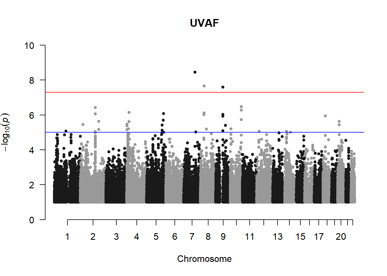

r_kvalV_mlma2 <- r_kvalV_mlma %>% filter(-log10(p)>1) %>% filter(Freq > 0.01)
manhattan(r_kvalV_mlma2, chr="Chr", bp="bp", p="p", snp="SNP", main = "R K-value V", ylim = c(0,10))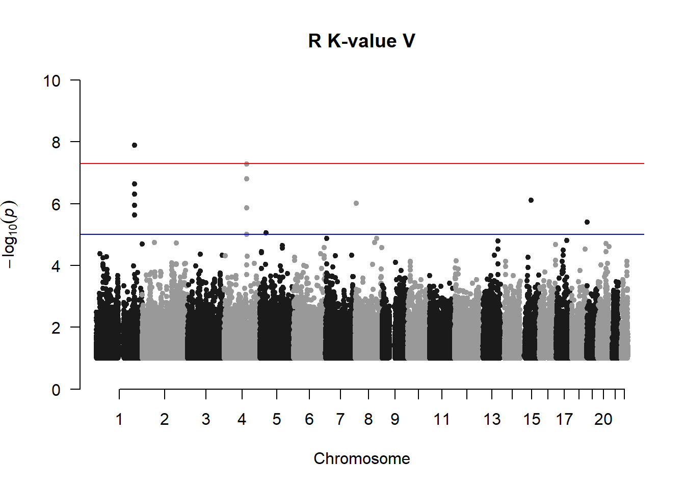

Filtering out the variants with MAF < 0.01 removes the lines of variants and produces manhattan plots that are more acceptable.

MLMA GWAS for most heritable trait