require(magrittr)

## Loading required package: magrittr

require(dplyr)

## Loading required package: dplyr

## 
## Attaching package: 'dplyr'

## The following objects are masked from 'package:stats':
## 
##     filter, lag

## The following objects are masked from 'package:base':
## 
##     intersect, setdiff, setequal, union

require(gaston)

## Loading required package: gaston

## Loading required package: Rcpp

## Loading required package: RcppParallel

## 
## Attaching package: 'RcppParallel'

## The following object is masked from 'package:Rcpp':
## 
##     LdFlags

## Gaston set number of threads to 2. Use setThreadOptions() to modify this.

## 
## Attaching package: 'gaston'

## The following object is masked from 'package:stats':
## 
##     sigma

## The following objects are masked from 'package:base':
## 
##     cbind, rbind

require(qqman)

## Loading required package: qqman

##

## For example usage please run: vignette('qqman')

##

## Citation appreciated but not required:

## Turner, S.D. qqman: an R package for visualizing GWAS results using Q-Q and manhattan plots. biorXiv DOI: 10.1101/005165 (2014).

##

## 
## Attaching package: 'qqman'

## The following object is masked from 'package:gaston':
## 
##     manhattan

Introduction

After running GWAS parallel in GCTA and gaston, we were concerned that GCTA was over burdening the test because the program was developed to deal with very large amounts of data. Considering our sample size was very small, random effects that may be in the GCTA models could have very significant effects on the GWAS results. This was evident on the manhattan plots generated for the same data, with the same adjustments between GCTA and gaston. In light of this, we have decided to move the GWAS analysis back to gaston.

I will be performing GWAS on 21 heritable traits (16 individual phenotypes and 5 principal components). I will be using the likelihood ratio test (LRT) as opposed to the wald test and score test as it is the most commonly used in GWAS and is suitable for smaller sample sizes (https://www.ncbi.nlm.nih.gov/pmc/articles/PMC4547377/). I will also be correcting for any effects of population stratification by including two prinicipal components as I have done with the heritability estimates.

For the Norfolk Island population, we set a genome-wide signficance threshold of p < 1.84e-7 rather than the general p < 5e-8 because that was calculated specifically for the sample size in the study.

Methods and Results

1. Load phenotypic data

nies_pheno_020918 <- read.csv('C:/Users/Martha/Documents/Honours/Project/honours.project/Data/nies_pheno_020918.csv', header = T)
head(nies_pheno_020918)

##   Fam.ID   UUID R.Logmar.VA L.Logmar.VA R.Sph..pre.dilate.
## 1      1 219960        0.02       -0.04               0.25
## 2      1 313180        0.10        0.16               0.00
## 3      1 320511       -0.06        0.02               1.00
## 4      1 400011       -0.14       -0.10               0.75
## 5      1 400013        0.30        0.30               1.50
## 6      1 316131        0.08        0.26               2.00
##   R.Cyl..pre.dilate. R.Axis..pre.dilate. L.Sph..pre.dilate.
## 1               0.00                   0               0.25
## 2              -0.75                  28              -0.50
## 3               0.00                   0               1.25
## 4              -0.25                 157               1.25
## 5              -0.25                  82               1.75
## 6              -1.00                  69               1.00
##   L.Cyl..pre.dilate. L.Axis..pre.dilate. R.K.value.H R.K.Value.H.Axis
## 1              -0.50                  79       42.00                2
## 2              -0.25                 164       41.25                7
## 3              -0.25                  29       42.50              177
## 4              -0.50                  20       42.50              165
## 5              -0.50                 100       43.00                0
## 6              -1.00                 114       42.75               63
##   R.K.value.V R.K.value.V.Axis L.K.value.H L.K.value.H.Axis L.K.value.V
## 1       43.00               92       42.50                5       43.50
## 2       42.25               97       41.50              168       42.00
## 3       43.50               87       42.00              170       42.50
## 4       43.25               75       42.75               17       43.25
## 5       43.00               90       42.75              111       43.00
## 6       44.00              153       43.00              115       43.50
##   L.K.value.V.Axis R.Pachimetry L.Pachimetry R.Axial.Length L.Axial.Length
## 1               95          532          554          24.31          24.10
## 2               78          608          612          25.02          25.21
## 3               80          499          512          23.37          23.65
## 4              107          602          601          23.32          23.34
## 5               21          552          550          22.93          22.70
## 6               25          583          588          23.49          23.54
##   R.AC.Depth L.AC.Depth R.IOP.mmHg L.IOP.mmHg R.CDR L.CDR totaluvafmm
## 1       3.09       3.03         14         14   0.9   0.9         0.0
## 2       3.38       3.92         16         15   0.9   0.7        74.4
## 3       3.29       3.08         17         18   0.4   0.4        27.5
## 4       3.81       3.83         15         17   0.6   0.6        47.0
## 5       3.22       3.13         18         18   0.4   0.4        20.1
## 6       3.24       3.04         12         12   0.3   0.3        12.9

2. Load genomic data (bed/bim/fam)

merged_nies_210818 <- read.bed.matrix("C:/Users/Martha/Documents/Honours/Project/honours.project/Data/merged_nies/merged_nies_geno_210818.bed")

## Reading C:/Users/Martha/Documents/Honours/Project/honours.project/Data/merged_nies/merged_nies_geno_210818.fam 
## Reading C:/Users/Martha/Documents/Honours/Project/honours.project/Data/merged_nies/merged_nies_geno_210818.bim 
## Reading C:/Users/Martha/Documents/Honours/Project/honours.project/Data/merged_nies/merged_nies_geno_210818.bed 
## ped stats and snps stats have been set. 
## 'p' has been set. 
## 'mu' and 'sigma' have been set.

3. Generate GRM, eigenK, and principal components

merged_nies_GRM <- GRM(merged_nies_210818)
merged_nies_eiK <- eigen(merged_nies_GRM)
merged_nies_eiK$values[ merged_nies_eiK$values < 0] <- 0
merged_nies_PC <- sweep(merged_nies_eiK$vectors, 2, sqrt(merged_nies_eiK$values), "*")

The genetic relationship matrix (GRM) will be used to account for the degree of relatedness among individuals, and the principal components will be used to correct for hiden population structure. Both of these ensure that any associations detected are not due to relatedness or hidden structures in the data i.e. they are true phenotypic-variant associations.

4. Perform GWAS on R K-value V (most heritable trait)

r_kvalV_gwas <- association.test(merged_nies_210818, nies_pheno_020918$R.K.value.V, method="lmm", test = "lrt", K = merged_nies_GRM, eigenK = merged_nies_eiK, p = 2)
r_kvalV_gwas <- na.omit(r_kvalV_gwas)
r_kvalV_gwas_filtered <- r_kvalV_gwas %>% filter(-log10(p)>1) %>% filter(freqA2 < 0.99)
qqman::manhattan(x = r_kvalV_gwas_filtered, chr = "chr", bp = "pos", p = "p", snp = "id", ylim = c(0,10), genomewideline = -log10(1.84e-7), main = "R K-value V", annotatePval = 1.84e-7)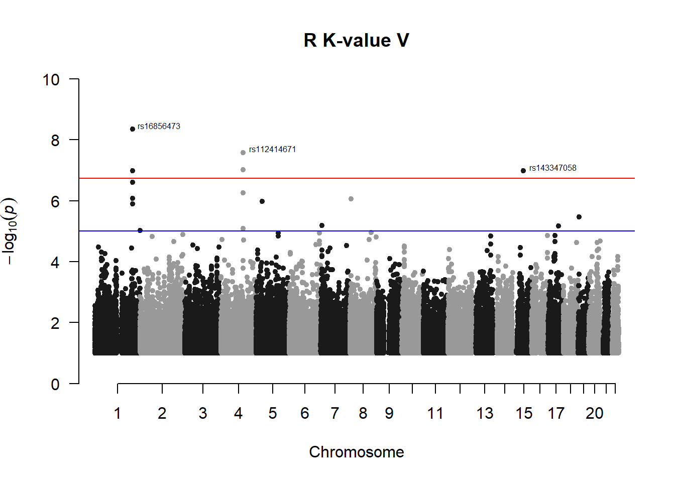

5. Repeat GWAS on other heritable traits

nies_heritable_pheno <- read.csv('C:/Users/Martha/Documents/Honours/Project/honours.project/Data/nies_heritable_pheno.csv', header = T)
head(nies_heritable_pheno)

##     UUID R.K.value.V L.Pachimetry coord.Dim.1 R.Pachimetry R.CDR
## 1 219960       43.00          554  -1.3318012          532   0.9
## 2 313180       42.25          612  -3.7993478          608   0.9
## 3 320511       43.50          512  -0.4961408          499   0.4
## 4 400011       43.25          601  -0.7904275          602   0.6
## 5 400013       43.00          550   0.4462229          552   0.4
## 6 316131       44.00          588   0.2319576          583   0.3
##   L.K.value.V R.Cyl..pre.dilate. L.CDR R.K.value.H coord.Dim.4 totaluvafmm
## 1       43.50               0.00   0.9       42.00   0.8399155         0.0
## 2       42.00              -0.75   0.7       41.25   2.0776045        74.4
## 3       42.50               0.00   0.4       42.50  -0.9796890        27.5
## 4       43.25              -0.25   0.6       42.50   1.5424175        47.0
## 5       43.00              -0.25   0.4       43.00   0.4965415        20.1
## 6       43.50              -1.00   0.3       42.75  -0.4216580        12.9
##   R.Axial.Length L.Axial.Length R.AC.Depth L.K.value.H L.AC.Depth
## 1          24.31          24.10       3.09       42.50       3.03
## 2          25.02          25.21       3.38       41.50       3.92
## 3          23.37          23.65       3.29       42.00       3.08
## 4          23.32          23.34       3.81       42.75       3.83
## 5          22.93          22.70       3.22       42.75       3.13
## 6          23.49          23.54       3.24       43.00       3.04
##   coord.Dim.7 R.IOP.mmHg coord.Dim.3 coord.Dim.8 L.IOP.mmHg
## 1   2.8552892         14  0.75849347  -1.0126837         14
## 2   2.2543673         16  0.41111735   0.3400838         15
## 3  -1.1828388         17 -0.62633667   0.1104747         18
## 4   2.2077992         15 -1.18429936   1.5903830         17
## 5  -0.5839491         18 -0.03864912  -0.2245313         18
## 6   1.1946733         12  0.16696557  -0.8347539         12

I compiled the data for the heritable traits into a new spreadsheet (loaded above).

pheno_gwas <- NULL
for (i in c(2:ncol(nies_heritable_pheno))){
  pheno_colnames <- colnames(nies_heritable_pheno[i])
  her_pheno_gwas <- association.test(merged_nies_210818, nies_heritable_pheno[,i], method = "lmm", 
                                     test = "lrt", K = merged_nies_GRM, eigenK = merged_nies_eiK, p =2)
  her_pheno_gwas <- na.omit(her_pheno_gwas)
  pheno_gwas_filtered <- her_pheno_gwas %>% filter(-log10(p)>1) %>% filter(freqA2 < 0.99)
  qqman::manhattan(x = pheno_gwas_filtered, chr = "chr", bp = "pos", p = "p", snp = "id", genomewideline = -log10(1.84e-7), main = paste(pheno_colnames))
  pheno_gwas <- pheno_gwas_filtered
}

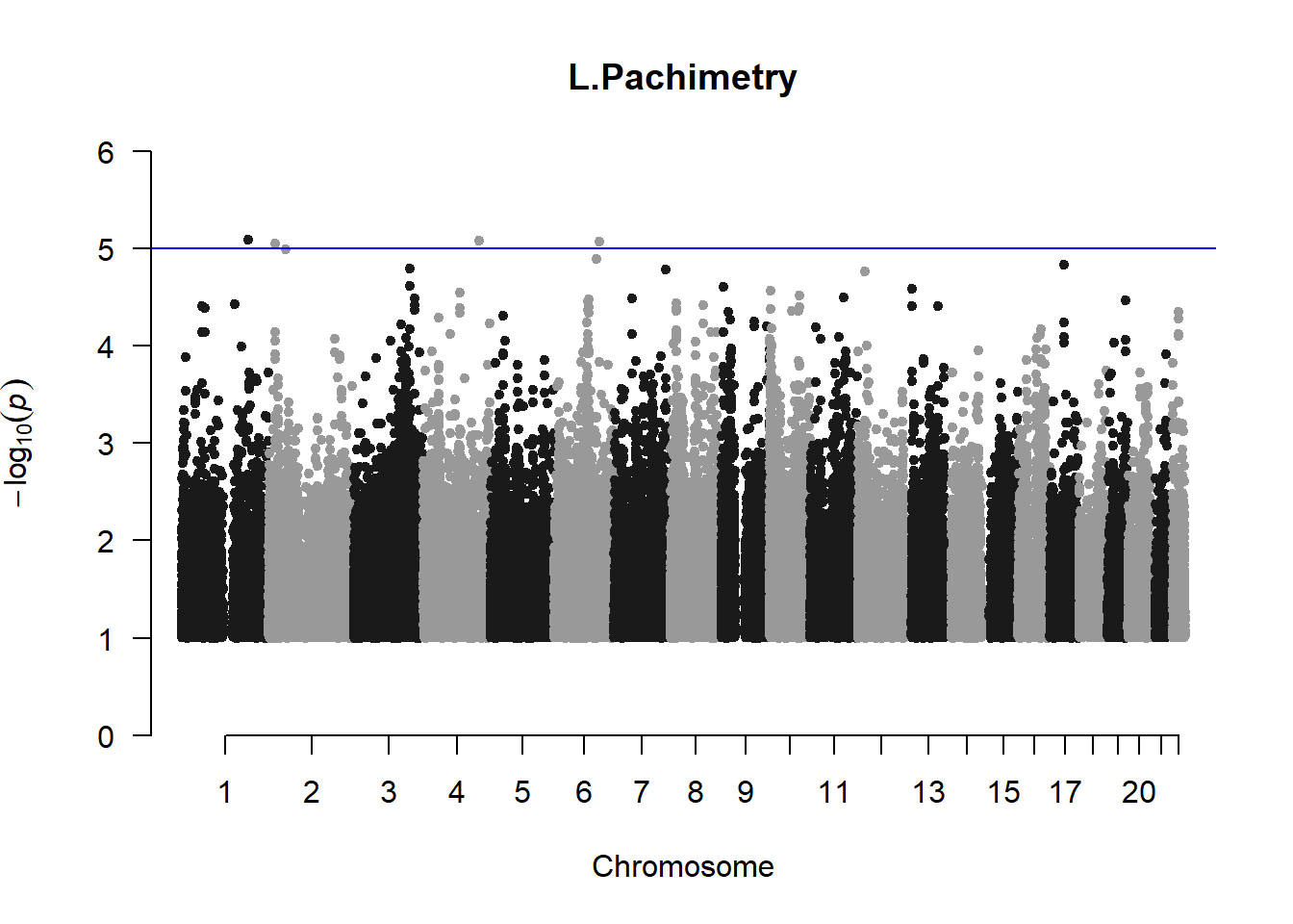
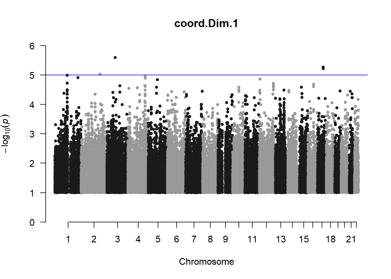
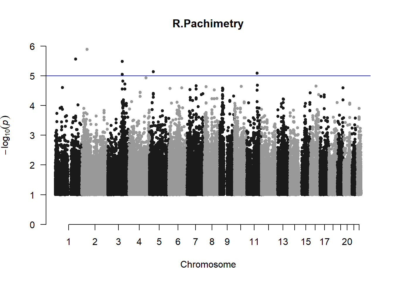
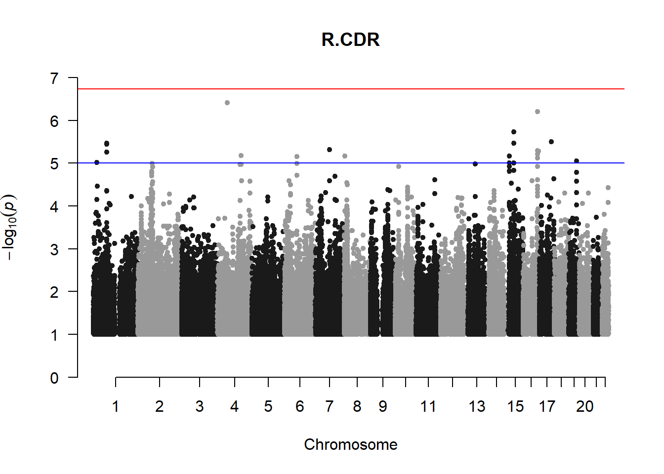
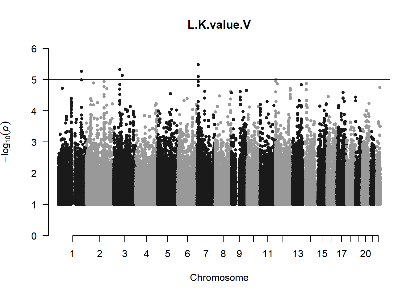
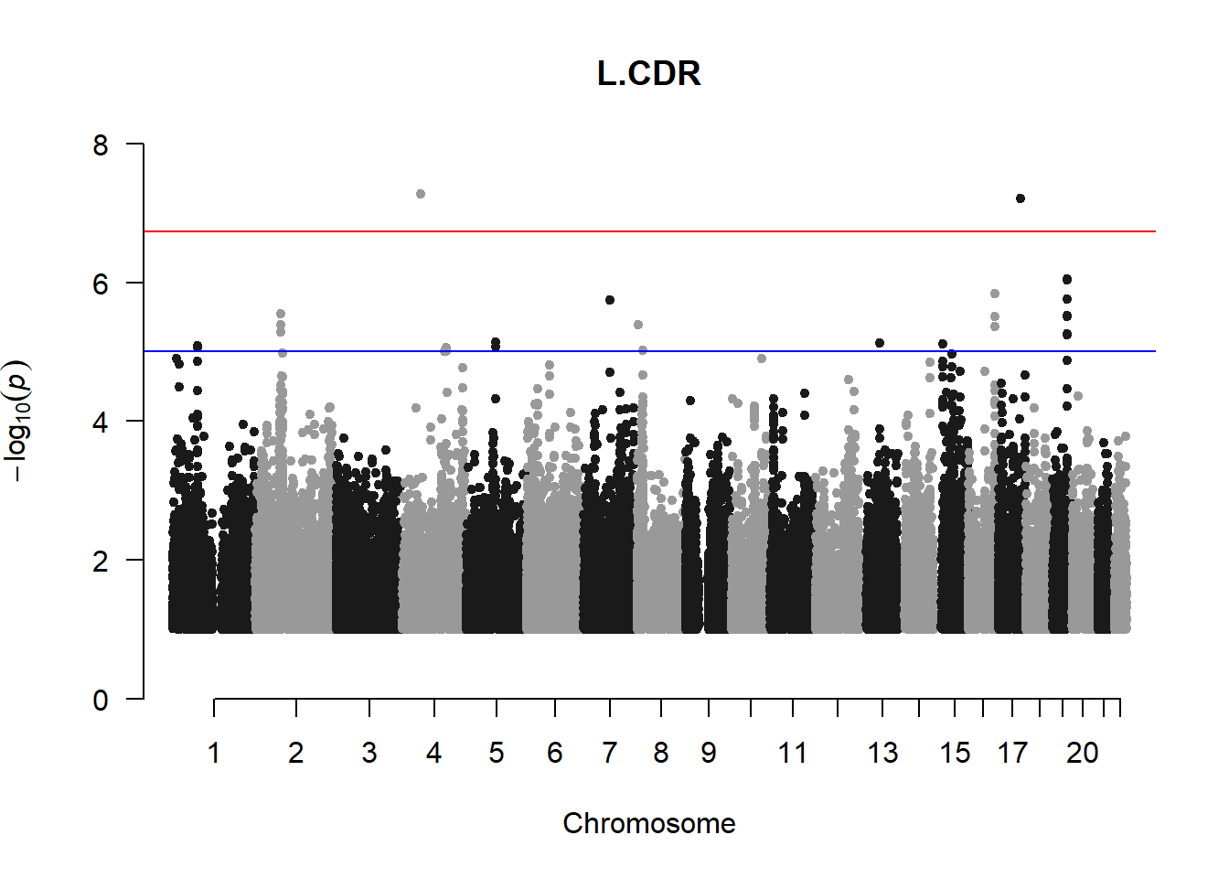
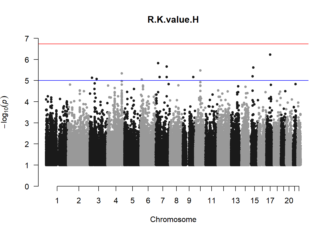
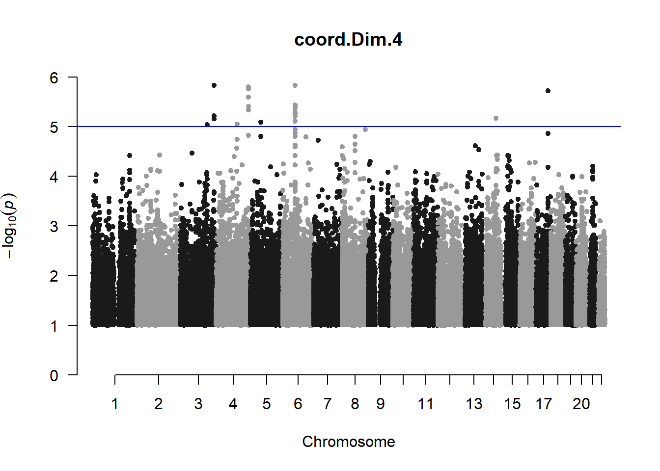
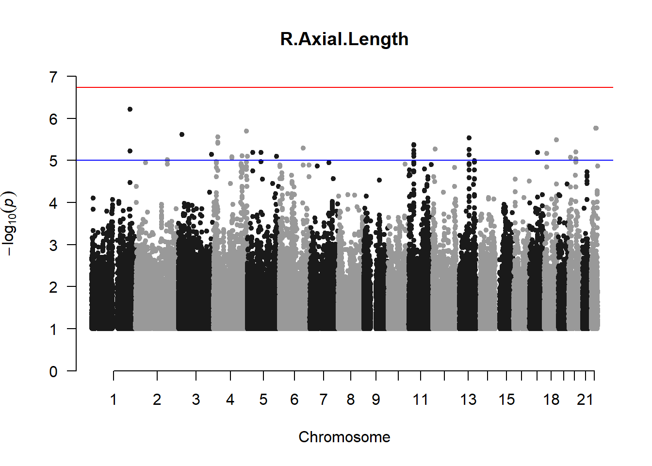
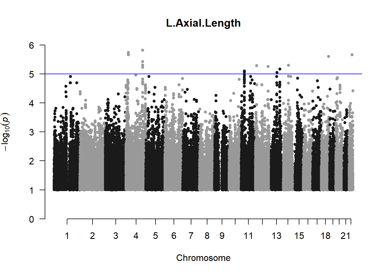
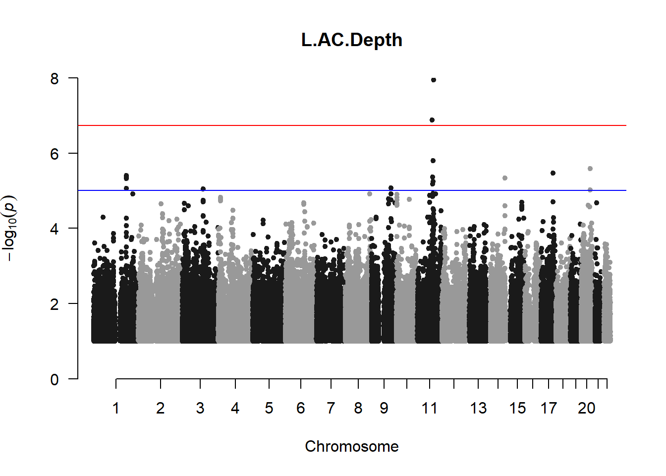
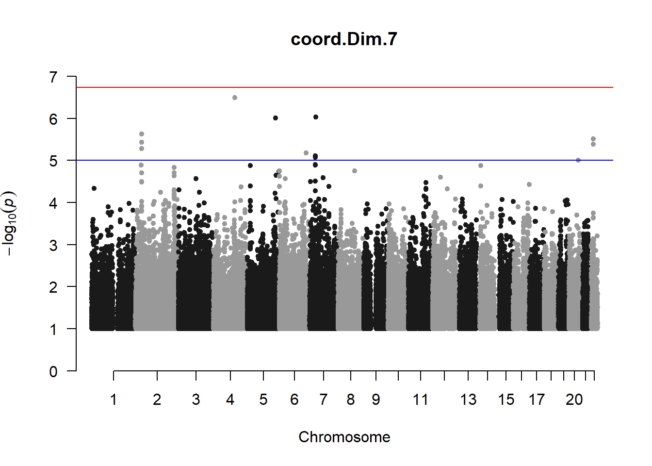
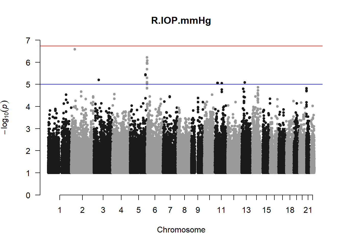
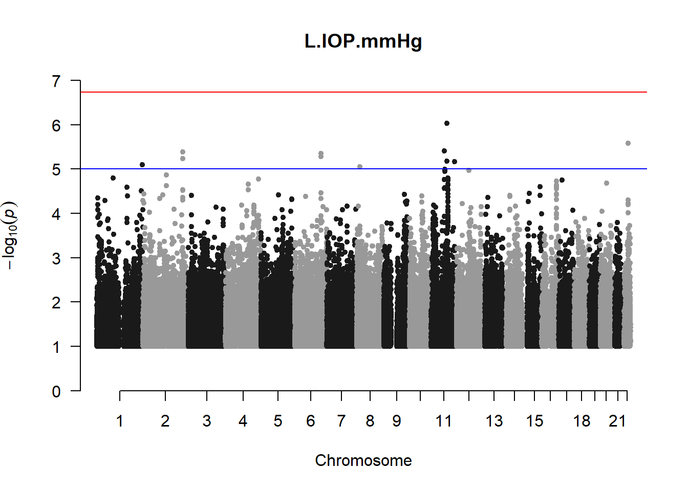
The loop above generates manhattan plots for the GWAS results of all 21 heritable traits.

6. Annotate manhattan plots with significant hits

I tried adding an annotation argument to the loop above to annotate hits that passed the genome-wide significance threshold. However, since not all manhattan plots had significant hits, the argument caused an error. I removed the argument from the loop and it was successful in generating all 21 manhattan plots. Of these, approximately 9 plots have significant hits and therefore require annotation.

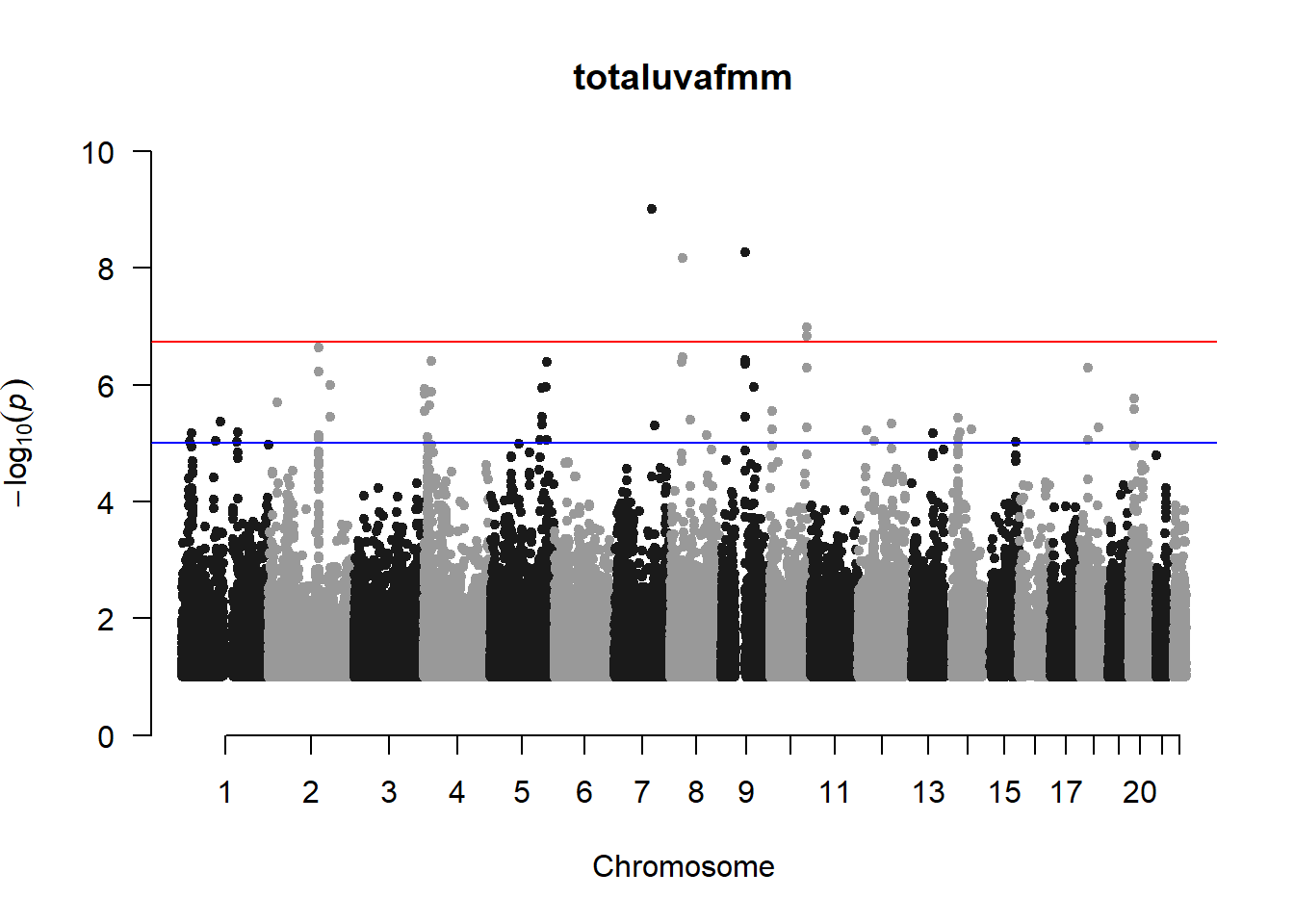
###uvaf
uvaf_gwas <- association.test(merged_nies_210818, nies_heritable_pheno$totaluvafmm, method="lmm", test = "lrt", K = merged_nies_GRM, eigenK = merged_nies_eiK, p = 2)
uvaf_gwas <- na.omit(uvaf_gwas)
uvaf_gwas_filtered <- uvaf_gwas %>% filter(-log10(p)>1) %>% filter(freqA2 < 0.99)
manhattan(x = uvaf_gwas_filtered, chr = "chr", bp = "pos", p = "p", snp = "id", ylim = c(0,10), genomewideline = -log10(1.84e-7), main = "Ultraviolet Autofluorescence", annotatePval = 1.84e-7)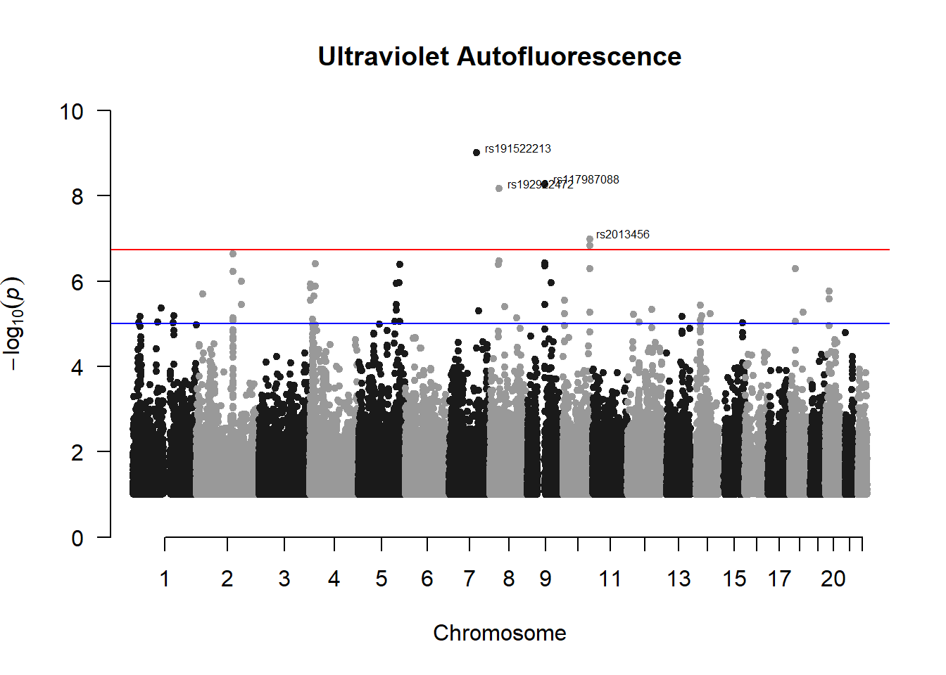

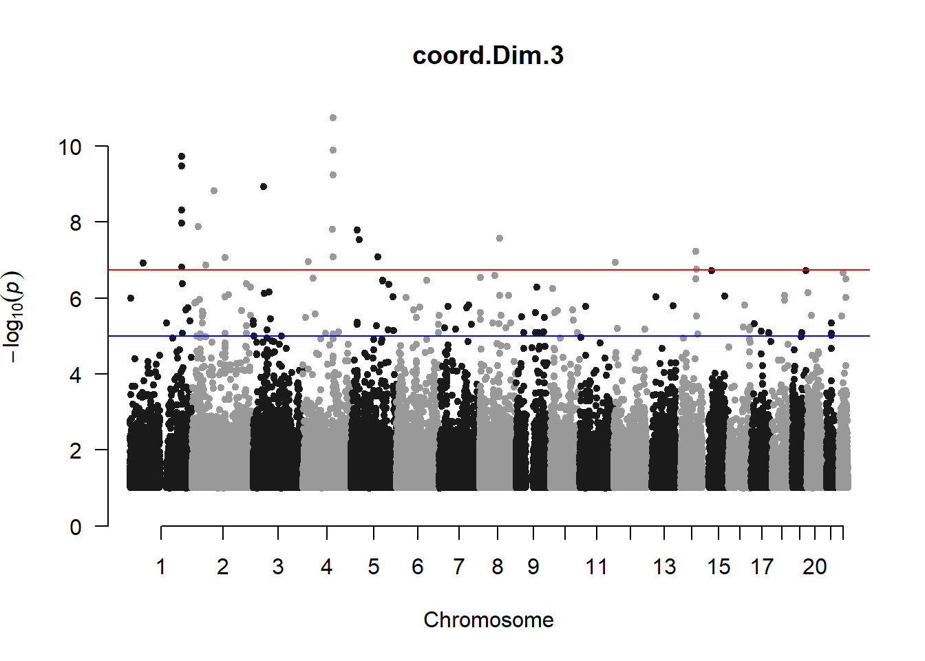
###PC3 
pc3_gwas <- association.test(merged_nies_210818, nies_heritable_pheno$coord.Dim.3, method="lmm", test = "lrt", K = merged_nies_GRM, eigenK = merged_nies_eiK, p = 2)
pc3_gwas <- na.omit(pc3_gwas)
pc3_gwas_filtered <- pc3_gwas %>% filter(-log10(p)>1) %>% filter(freqA2 < 0.99)
manhattan(x = pc3_gwas_filtered, chr = "chr", bp = "pos", p = "p", snp = "id", ylim = c(0,10), genomewideline = -log10(1.84e-7), main = "Component 3", annotatePval = 1.84e-7)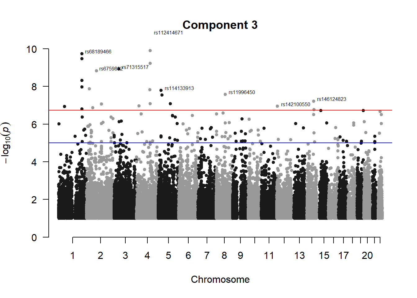

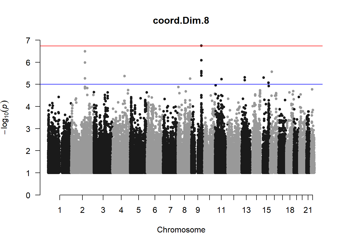
###PC8
pc8_gwas <- association.test(merged_nies_210818, nies_heritable_pheno$coord.Dim.8, method="lmm", test = "lrt", K = merged_nies_GRM, eigenK = merged_nies_eiK, p = 2)
pc8_gwas <- na.omit(pc8_gwas)
pc8_gwas_filtered <- pc8_gwas %>% filter(-log10(p)>1) %>% filter(freqA2 < 0.99)
manhattan(x = pc8_gwas_filtered, chr = "chr", bp = "pos", p = "p", snp = "id", ylim = c(0,10), genomewideline = -log10(1.84e-7), main = "Component 8", annotatePval = 1.84e-7)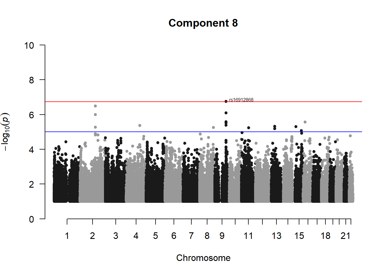

###L ACD
l_acd_gwas <- association.test(merged_nies_210818, nies_heritable_pheno$L.AC.Depth, method="lmm", test = "lrt", K = merged_nies_GRM, eigenK = merged_nies_eiK, p = 2)
l_acd_gwas <- na.omit(l_acd_gwas)
l_acd_gwas_filtered <- l_acd_gwas %>% filter(-log10(p)>1) %>% filter(freqA2 < 0.99)
manhattan(x = l_acd_gwas_filtered, chr = "chr", bp = "pos", p = "p", snp = "id", ylim = c(0,10), genomewideline = -log10(1.84e-7), main = "Left Anterior Chamber Depth", annotatePval = 1.84e-7)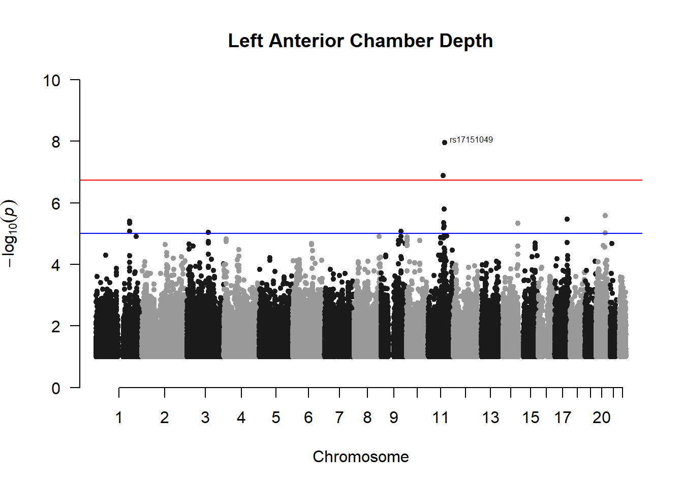

###L CDR
l_cdr_gwas <- association.test(merged_nies_210818, nies_heritable_pheno$L.CDR, method="lmm", test = "lrt", K = merged_nies_GRM, eigenK = merged_nies_eiK, p = 2)
l_cdr_gwas <- na.omit(l_cdr_gwas)
l_cdr_gwas_filtered <- l_cdr_gwas %>% filter(-log10(p)>1) %>% filter(freqA2 < 0.99)
manhattan(x = l_cdr_gwas_filtered, chr = "chr", bp = "pos", p = "p", snp = "id", ylim = c(0,10), genomewideline = -log10(1.84e-7), main = "Left Cup-to-Disc Ratio", annotatePval = 1.84e-7)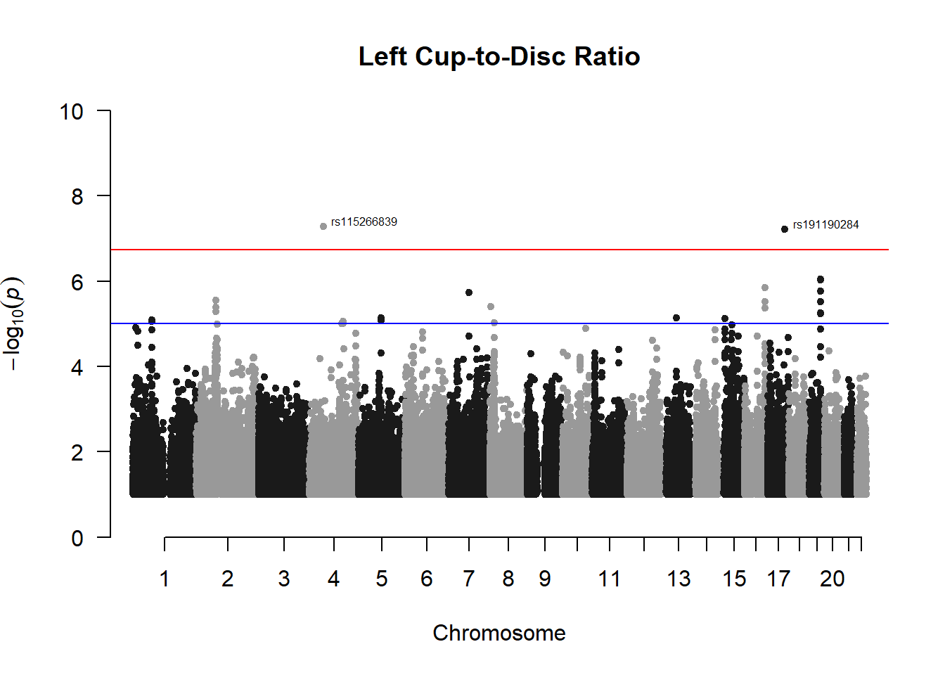

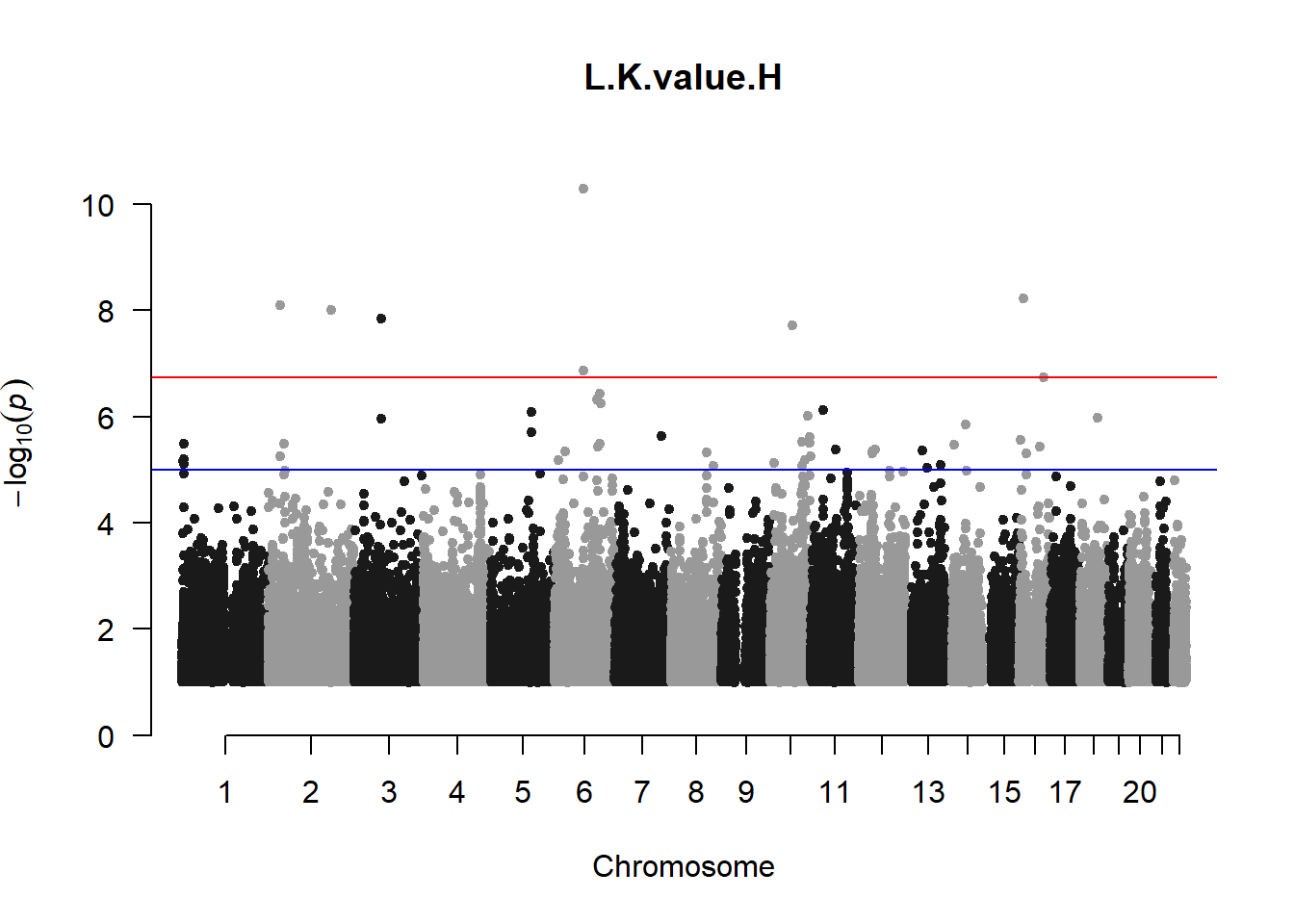
###L Kval H
l_KvalH_gwas <- association.test(merged_nies_210818, nies_heritable_pheno$L.K.value.H, method="lmm", test = "lrt", K = merged_nies_GRM, eigenK = merged_nies_eiK, p = 2)
l_KvalH_gwas <- na.omit(l_KvalH_gwas)
l_KvalH_gwas_filtered <- l_KvalH_gwas %>% filter(-log10(p)>1) %>% filter(freqA2 < 0.99)
manhattan(x = l_KvalH_gwas_filtered, chr = "chr", bp = "pos", p = "p", snp = "id", ylim = c(0,10), genomewideline = -log10(1.84e-7), main = "Left Horizontal K-value", annotatePval = 1.84e-7)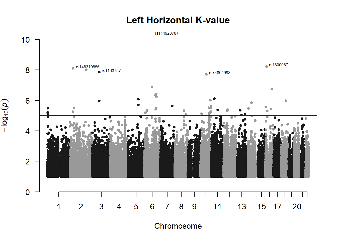

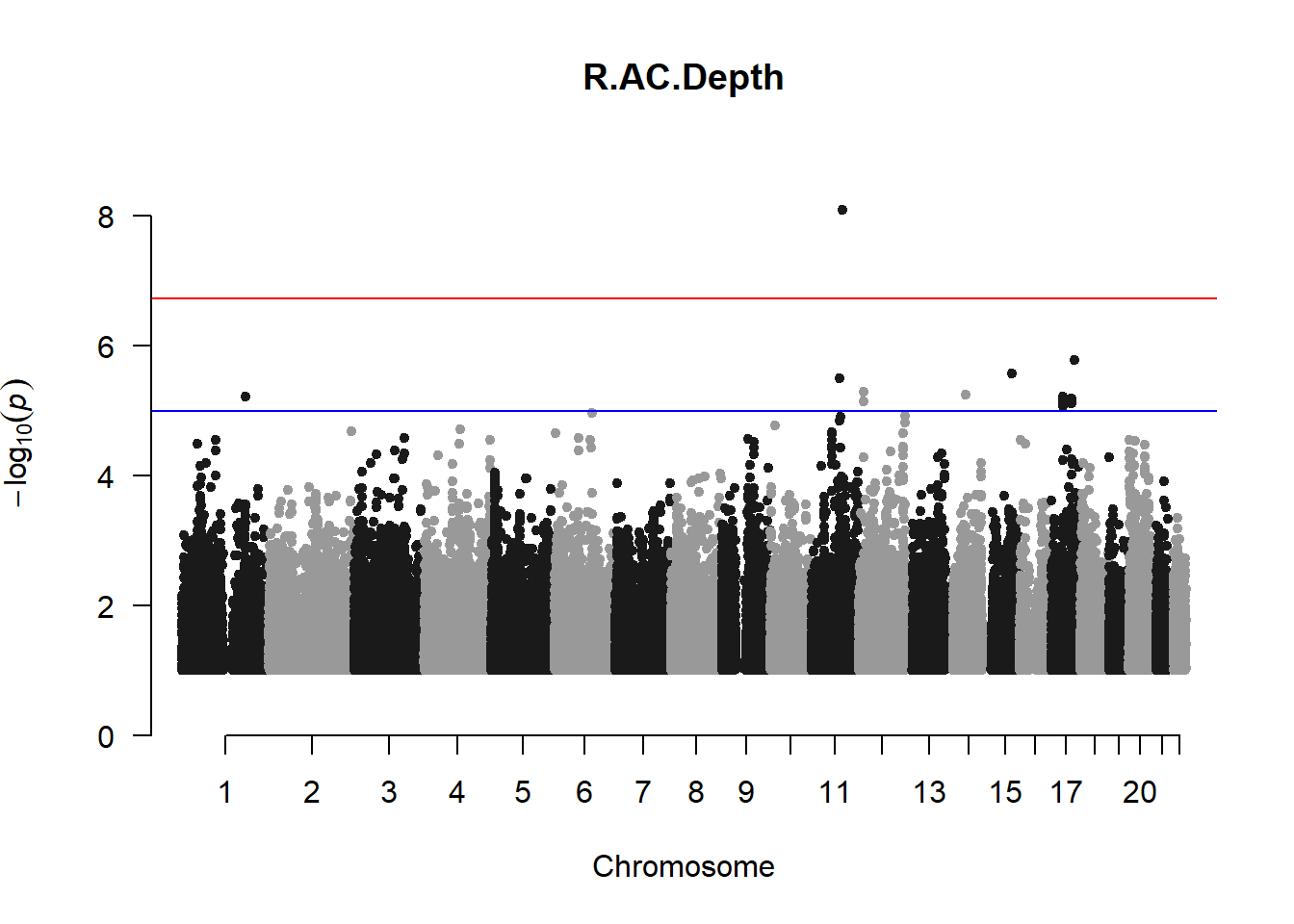
###R ACD 
r_acd_gwas <- association.test(merged_nies_210818, nies_heritable_pheno$R.AC.Depth, method="lmm", test = "lrt", K = merged_nies_GRM, eigenK = merged_nies_eiK, p = 2)
r_acd_gwas <- na.omit(r_acd_gwas)
r_acd_gwas_filtered <- r_acd_gwas %>% filter(-log10(p)>1) %>% filter(freqA2 < 0.99)
manhattan(x = r_acd_gwas_filtered, chr = "chr", bp = "pos", p = "p", snp = "id", ylim = c(0,10), genomewideline = -log10(1.84e-7), main = "Right Anterior Chamber Depth", annotatePval = 1.84e-7)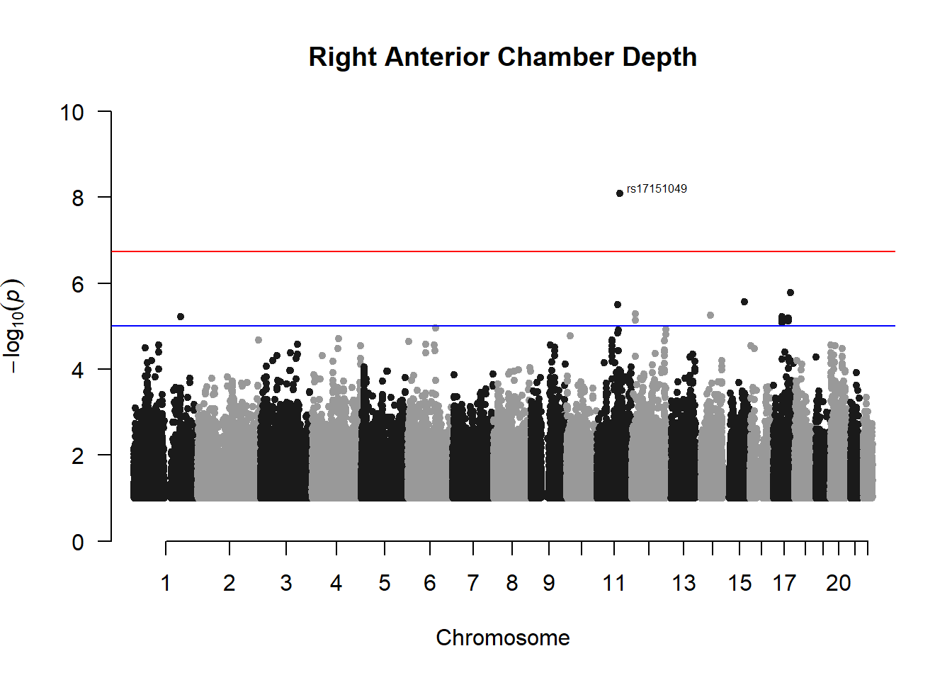

###R Cyl
r_cyl_gwas <- association.test(merged_nies_210818, nies_heritable_pheno$R.Cyl..pre.dilate, method="lmm", test = "lrt", K = merged_nies_GRM, eigenK = merged_nies_eiK, p = 2)
r_cyl_gwas <- na.omit(r_cyl_gwas)
r_cyl_gwas_filtered <- r_cyl_gwas %>% filter(-log10(p)>1) %>% filter(freqA2 < 0.99)
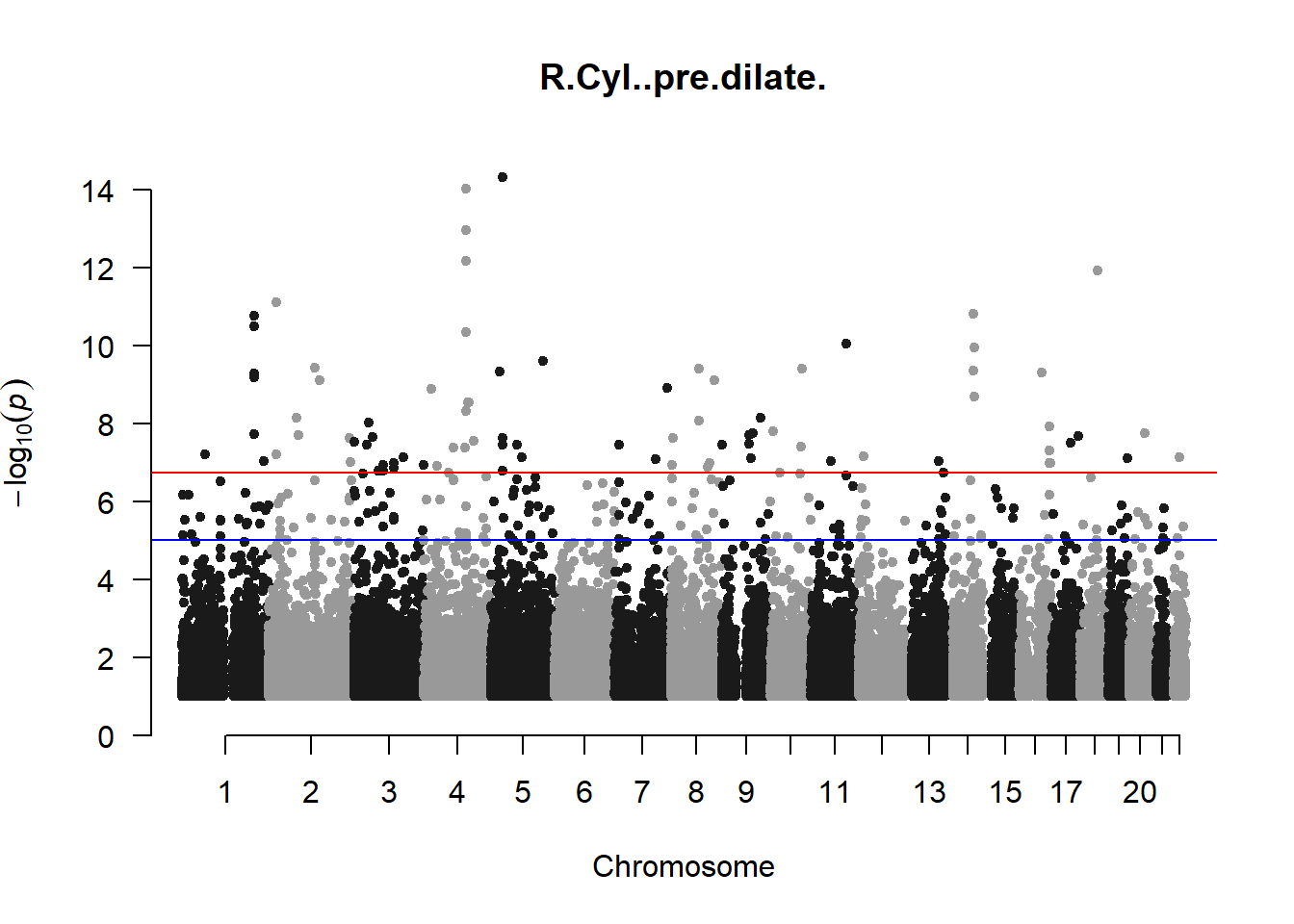
manhattan(x = r_cyl_gwas_filtered, chr = "chr", bp = "pos", p = "p", snp = "id", ylim = c(0,15), genomewideline = -log10(1.84e-7), main = "Right Cylindrical Pre-Dilate Refractive Error", annotatePval = 1.84e-7)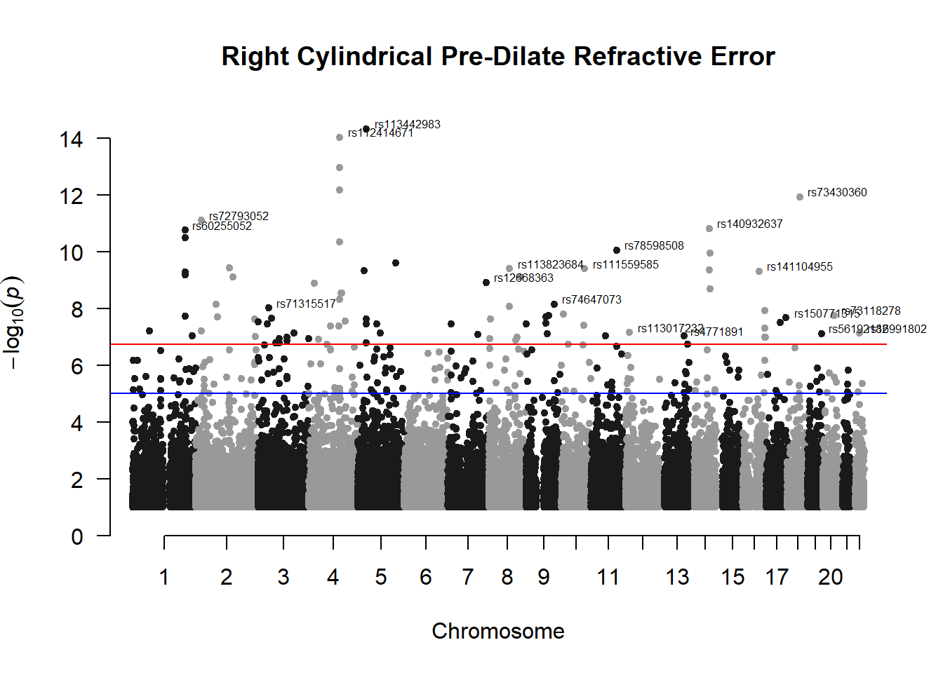

These manhattan plots display significant SNPs that pass the genome-wide significance threshold. Although this indicates significant association with traits, they may not all be “true”. Typically, robust associations, or significant results have supporting SNPs surrounding the most significant peak. Therefore, I will apply a filter on these results.

Performing GWAS on heritable traits