| tags: [ R Data Cleaning ] categories: [Coding ]
Plotting histograms for quantitative phenotypic data
Introduction
Histograms show the frequency distribution of continuous data. It can also be used to inspect whether the data is normally distributed, skewed, and indicate the presence of outliers or non-sense data. The continuous data is split into intervals called bins, and the frequency of scores that fit within each bin is recorded and plotted. Since the data is continuous, histograms are plotted with no spaces in between each bar. (https://statistics.laerd.com/statistical-guides/understanding-histograms.php)
Aim
To plot histograms for all continuous phenotypic variables.
Methods and results
- Identify all continuous variables in the phenotypic dataset by inspection.
- Plot histograms
- The simplest method to plot histograms is as follows:
phen.data <- read.csv('C:/Users/Martha/Documents/Honours/Project/honours.project/Data/NIES_master_database.csv')
hist.height <- hist(phen.data$Current.height)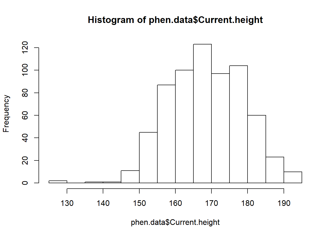 - In the case above, the histogram was attributed to the object ‘hist.height’ so that it can be viewed later without having to run the line of code. - Using the hist() function for each variable would mean extensive repetition of the same code and would be time consuming. Therefore, I attempted to build an appropriate script that would plot all of the histograms without repeating the code.
b. Before creating the script that would plot the histograms, I created a subset of data that contained only continuous variables. #select the column headings that contain continous data
quant.data <- c("Current.height", "Current.weight", "Logmar.VA.Right", "RVA.with.PH", "Logmar.VA.Left", "LVA.with.PH",
"R.Sph..pre.dilate.", "R.Cyl..pre.dilate.", "R.Axis..pre.dilate.", "L.Sph..pre.dilate.", "L.Cyl..pre.dilate.",
"L.Axis..pre.dilate.", "R.K.value.H", "R.K.Value.H.Axis", "R.K.value.V", "R.K.value.V.Axis", "L.K.value.H",
"L.K.value.H.Axis", "L.K.value.V", "L.K.value.V.Axis", "Lang.score", "R.Pachimetry", "L.Pachimetry", "R.Axial.Length",
"L.Axial.Length", "AC.Depth.R", "AC.Depth.L", "R.IOP.mmHg", "L.IOP.mmHg", "CDR.RE", "CDR.LE")
#subset the continuous data
quant.data.subset <- phen.data[quant.data]
#check the output
head(quant.data.subset)## Current.height Current.weight Logmar.VA.Right RVA.with.PH Logmar.VA.Left
## 1 NA NA 0.02 0.02 -0.04
## 2 170 78 0.10 0.10 0.16
## 3 180 86 0.00 0.00 0.00
## 4 183 NA 0.30 0.10 0.08
## 5 NA 69 0.00 0.00 -0.10
## 6 162 NA 0.24 0.16 0.36
## LVA.with.PH R.Sph..pre.dilate. R.Cyl..pre.dilate. R.Axis..pre.dilate.
## 1 -0.04 0.25 0.00 0
## 2 0.10 0.00 -0.75 28
## 3 0.00 1.25 -1.25 148
## 4 0.08 1.25 -0.25 97
## 5 -0.10 1.25 -0.25 37
## 6 0.14 4.00 -0.50 46
## L.Sph..pre.dilate. L.Cyl..pre.dilate. L.Axis..pre.dilate. R.K.value.H
## 1 0.25 -0.50 79 42.00
## 2 -0.50 -0.25 164 41.25
## 3 1.25 -0.25 24 NA
## 4 1.50 -0.50 81 44.75
## 5 1.25 -0.75 164 44.75
## 6 3.75 -0.75 180 42.00
## R.K.Value.H.Axis R.K.value.V R.K.value.V.Axis L.K.value.H
## 1 2 43.00 92 42.50
## 2 7 42.25 97 41.50
## 3 NA NA NA NA
## 4 5 45.00 95 45.00
## 5 0 44.75 90 44.25
## 6 8 43.25 98 42.25
## L.K.value.H.Axis L.K.value.V L.K.value.V.Axis Lang.score R.Pachimetry
## 1 5 43.50 95 550 532
## 2 168 42.00 78 550 608
## 3 NA NA NA 550 507
## 4 60 45.25 150 NA 560
## 5 178 44.75 88 550 556
## 6 177 43.25 87 550 498
## L.Pachimetry R.Axial.Length L.Axial.Length AC.Depth.R AC.Depth.L
## 1 554 24.31 24.10 3.09 3.03
## 2 612 25.02 25.21 3.38 3.92
## 3 510 22.78 22.80 3.40 3.45
## 4 559 23.02 22.98 3.00 2.85
## 5 562 21.75 22.04 2.60 2.53
## 6 501 23.06 23.17 2.94 3.04
## R.IOP.mmHg L.IOP.mmHg CDR.RE CDR.LE
## 1 14 14 0.9 0.9
## 2 16 15 0.9 0.7
## 3 26 22 0.7 0.7
## 4 14 14 0.2 0.2
## 5 22 21 0.3 0.3
## 6 18 20 0.6 0.6- Only the results from the first 6 individuals are shown above to provide an example of the output. 31 quantitative variables were selected from the phenotypic dataset. Although there are more, any quantitative variable with more than 400 missing cells were excluded. That said, most of the excluded variables had very few (<5) data points present and will most likely not be usable for subsequent analysis, and cannot be imputed correctly.
- The following script was used to plot all histograms in a panel:
#install the necessary packages
install.packages('tidyverse', dependencies = TRUE, repos = "http://cran.us.r-project.org" )
## Installing package into 'C:/Users/Martha/Documents/R/win-library/3.4'
## (as 'lib' is unspecified)## package 'tidyverse' successfully unpacked and MD5 sums checked
##
## The downloaded binary packages are in
## C:\Users\Martha\AppData\Local\Temp\Rtmp4qKD2S\downloaded_packagesrequire(tidyverse)## Loading required package: tidyverse## -- Attaching packages ------------------------------------------------------------------------------------- tidyverse 1.2.1 --## v ggplot2 2.2.1 v purrr 0.2.4
## v tibble 1.4.2 v dplyr 0.7.4
## v tidyr 0.8.0 v stringr 1.2.0
## v readr 1.1.1 v forcats 0.2.0## -- Conflicts ---------------------------------------------------------------------------------------- tidyverse_conflicts() --
## x dplyr::filter() masks stats::filter()
## x dplyr::lag() masks stats::lag()install.packages('ggplot2', dependencies = TRUE, repos = "http://cran.us.r-project.org")## Installing package into 'C:/Users/Martha/Documents/R/win-library/3.4'
## (as 'lib' is unspecified)## Warning: package 'ggplot2' is in use and will not be installedrequire(ggplot2)
#plot histograms
quant.data.subset %>%
keep(is.numeric) %>%
gather() %>%
ggplot(aes(value)) + facet_wrap(~ key, scales = "free") + geom_histogram(fill = 'grey', colour = "black")## `stat_bin()` using `bins = 30`. Pick better value with `binwidth`.## Warning: Removed 1165 rows containing non-finite values (stat_bin).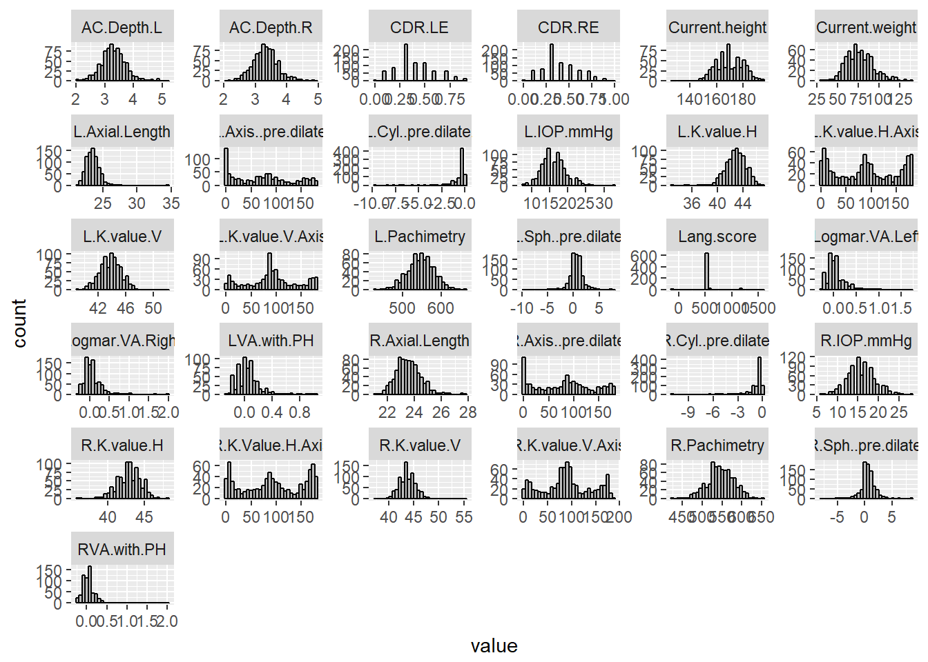
Discussion
The script I used to plot the histograms was sourced from (https://drsimonj.svbtle.com/quick-plot-of-all-variables). Prior to this, I considered using a ‘for’ loop, an ‘apply’ function, or the ‘repeat’ function to iterate the histogram command. These proved to be more complex than necessary, or were not applicable to this dataset.
The results of the histograms show the frequency distributions of the scores of each quantitative variable. From inspection, there does not seem to be non-sense data present, except for ‘Lang.score’ which shows a large peak at 550, and smaller peaks at -99, 600, and 1200. The peaks at 550“, 600”, and 1200" were expected, as these are the set disparities from the stereoscropic test (https://www.lang-stereotest.com/pages/video, https://cdn.shopify.com/s/files/1/0984/9292/files/Brief_Instructions_English_4_Pages_PDF.pdf?1321875810004346330, [paper describing NIES methods]). However, there were a few datapoints at -99, and upon inspection of the dataset, there was one point at 0, and a couple at 1300. These seem to be non-sense data, because it does not fit the categories. They may have been typographical errors during data entry. Although the -99 may be legitimate entries as they appear several times.
Evidently, it is difficult to determine with certainty, which, if there are any, are the outliers in each variable. It may be worthwhile following this with the identification of outliers using the boxplot.stats() function. Additionally, from an initial inspection of the dataset, there are a few individuals with systematically missing data. Some of these individuals appear to have most of the quantitative data, but lack environmental or demographic data, some are vice versa, and two appear to have almost all of the data missing (all of these individuals are highlighted in the excel file).