Introduction

The final step to the second part of aim 1 is to perform a PCA on the genomic data to investigate the population structure. This is important because it will allow me to determine if there are any underlying genetic structures in the genomic data and I can account for relatedness among individuals for subsequent analyses.

Methods and Results

1. Run PCA

plink1.9 --bfile merged_nies --pca 180 var-wts --out plink_output/nies_final_pca

The count had to be increased (default is 20) because there are over 100 components with an eigenvalue >1.

Including the var-wts modifier will generate a file for variant weights.

2. Load eigenvalue results

nies_final_pca_eigenval <- read.table('C:/Users/Martha/Documents/Honours/Project/honours.project/Data/plink_output/nies_final_pca.eigenval', header = F)

head(nies_final_pca_eigenval)

##        V1
## 1 4.25322
## 2 3.95956
## 3 3.18262
## 4 2.86084
## 5 2.80460
## 6 2.73255

3. Produce screeplot

barplot(nies_final_pca_eigenval$V1, 
        names.arg = 1:nrow(nies_final_pca_eigenval), 
        main = "NIES PCA Eigenvalue",
        xlab = "Principal Components",
        ylab = "Eigenvalue",
        col ="lightskyblue2")
lines(x = 1:nrow(nies_final_pca_eigenval), nies_final_pca_eigenval$V1, 
      type = "b", pch = 19, col = "red")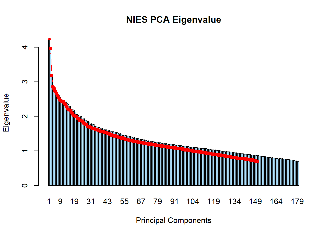

There are 124 principal components that have an eigenvalue >1.

Performing PCA on genomic data

Introduction

Methods and Results

1. Run PCA

2. Load eigenvalue results

3. Produce screeplot