Introduction

Applying a missing genotype filter for individuals and markers (described in previous entry) yielded unexpected results as a significant number of individuals and variants were removed. Considering the high genotyping rates (~99%) of the original files (WGS and SNP-array), there should only be a small number of variants removed due to missing genotypes.

This exercise is aimed at determining the possible cause for this filtering issue by testing the filtering parameters on the original data set and merged data set. This should identify the step at which the genotyping rate changes.

Note: this exercise was performed on taurus #Methods and Results ###1. Apply missingness filters on original WGS data set

plink --bfile NI_wgs_merged_snps --mind 0.05 --make-bed -out test_output/wgs_imiss_filter

Output: No individuals were removed.

plink --bfile NI_wgs_merged_snps --geno 0.1 --make-bed -out test_output/wgs_imiss_filter

Output: 1 variant removed

plink --bfile NI_wgs_merged_snps --geno 0.01 --make-bed --out test_output/wgs_imiss_filter

Output: 781,724 variants removed (18,426,862 variants remain)

2. Apply missingness filters on original SNP-array data set

plink --bfile NI.snp.hg38_final --mind 0.05 --make-bed --out test_output/array_imiss_filter

Output: No individuals were removed.

plink --bfile NI.snp.hg38_final --geno 0.1 --make-bed -out test_output/array_imiss_filter

output: 810,752 variants removed (25,244,548 variants remain)

plink --bfile NI.snp.hg38_final --geno 0.01 --make-bed --out test_output/array_imiss_filter

Output: 4,554,230 variants removed (21,501,070 variants remain)

3. Apply missingness filters on merged data set

plink --bfile plink_output/filtered_merge --mind 0.05 --make-bed --out test_output/merged_miss_filter

Output: 96 individuals removed (424 individuals remain)

plink --bfile plink_output/filtered_merge --mind 0.1 --make-bed --out test_output/merged_miss_filter

Output: 94 individuals removed (426 individuals remain)

plink --bfile plink_output/filtered_merge --geno 0.01 --make-bed --out test_output/merged_miss_filter

Output: 8,003,914 variants removed (1,151,139 variants remain)

plink --bfile plink_output/filtered_merge --geno 0.1 --make-bed --out test_output/merged_miss_filter

Output: 2,857,039 variants removed (6,298,014 variants remain)

Applying the filtering parameters on the merged data set indicates that the change in the genotyping rates occurred because of this merge. From the PLINK manual (http://zzz.bwh.harvard.edu/plink/dataman.shtml#merge), it appears that the default merge mode uses a consensus. This means that if there is a missing genotype in one file, it is overwritten by the other file. However, if a genotype is present in both files but they mismatch, it is treated as missing.

4. Re-run merge-mode 6 to determine mismatching calls between the two files.

plink --bfile plink_output/wgs_filtered --bmerge plink_output/array_filtered.bed plink_output/array_filtered.bim plink_output/array_filtered.fam --merge-mode 6 --out plink_output/merged_mode6_filtered

Output: - 860,574,982 overlapping calls - 835,821,129 non-missing in both filesets - 579,288,999 concordant - 69.31% concordance rate

This low concordance rate indicates that there is a substantial number of calls between the file sets that mismatch. Therefore, merging them using the default setting would identify these calls as missing, which explains the large number of individuals and variants filtered out.

5. Use merge-mode 3 to merge the file sets.

plink --bfile plink_output/array_filtered --bmerge plink_output/wgs_filtered.bed plink_output/wgs_filtered.bim plink_output/wgs_filtered.fam --merge-mode 3 --make-bed --out plink_output/filtered_merge_mode3

Output: - 9,155,053 variants and 520 individuals pass filters and QC - total genotyping rate = 97.7%

Already, this total genotyping rate has increased compared to using the default merge setting (~92%).

6. Generate allele frequency stats

plink1.9 --bfile plink_output/filtered_merge_mode3 --freq --out plink_output/merged_mode3_freq

7. Load allele freq file

merged_mode3_freq <- read.table('C:/Users/Martha/Documents/Honours/Project/honours.project/Data/plink_output/merged_mode3_freq.frq', header = T)

8. Generate histogram for allele frequency distributions

hist(merged_mode3_freq$MAF, main = "Allele Frequency Distributions of Merged Data Set (Mode3)", xlab = "Minor Allele Frequency", xlim = c(0.0, 0.5), col = "turquoise3")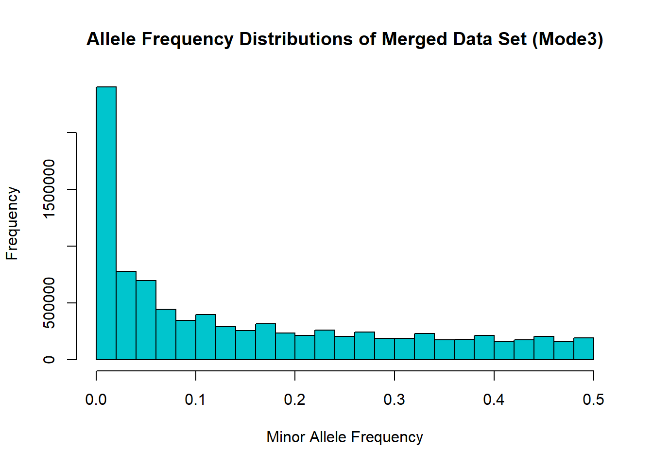

9. Filter out variants based on HWE p-value

plink1.9 --bfile plink_output/filtered_merge_mode3 --hwe 1.8e-7 --make-bed --out plink_output/merged_hwe_filter

Output: - 2295 variants removed due to HWE p-value - 9,152,758 variants remain

10. Load spreadsheet with NI study participants

ni_ped_uuid <- read.csv('C:/Users/Martha/Documents/Honours/Project/honours.project/Data/NI_UUID_Ped_20180718.csv', header = T) 

head(ni_ped_uuid)

##     UUID Ped_ID LAB_ID  PID  SID NIES KCCGID Gender        DOB IN_2000
## 1 110020     NA   1002 <NA> <NA> <NA>   <NA> Female  5/16/1929       1
## 2 110030     NA   1003 <NA> <NA> <NA>   <NA> Female  5/23/1928       1
## 3 110040   3676   1004 <NA> <NA> <NA>   <NA> Female  2/08/1959       1
## 4 110050    765   1005 <NA> <NA> <NA>   <NA>   Male 11/07/1954       1
## 5 110080     NA   1008 <NA> <NA> <NA>   <NA> Female 10/07/1933       1
## 6 110090     NA   1009 <NA> <NA> <NA>   <NA> Female 10/08/1968       1
##   AGE_2000NIHS IN_2010 AGE_2010NIHS IN_NIES AGE_NIES RECOLLECT COREPED_1
## 1           71       0           80       0       79         0         0
## 2           72       0           81       0       80         0         0
## 3           41       0           50       0       49         0         0
## 4           46       0           55       0       54         0         1
## 5           67       0           76       0       75         0         0
## 6           32       0           41       0       40         0         0
##   COREPED_2 Miles_core DNA_NIHS X2000NIHS_GWAS X2010NIHS_GWAS GWAS_NIHS
## 1         0          0        1              0              0         0
## 2         0          0        1              0              0         0
## 3         0          0        1              0              0         0
## 4         1          1        1              1              0         1
## 5         0          0        1              0              0         0
## 6         0          0        1              0              0         0
##   DNA_NIES GWAS_NIES Total_GWAS NI_exprs WGS_data DNA_TOTAL
## 1        0         0          0        0        0         1
## 2        0         0          0        0        0         1
## 3        0         0          0        0        0         1
## 4        0         0          1        0        0         1
## 5        0         0          0        0        0         1
## 6        0         0          0        0        0         1
##   Relation.to.NIHS.Pedigree..n.6379. patID matID Ped_Gender isParent
## 1                               <NA>    NA    NA       <NA>       NA
## 2                               <NA>    NA    NA       <NA>       NA
## 3                               <NA>    NA    NA       <NA>       NA
## 4                               <NA>   764   762       Male    FALSE
## 5                               <NA>    NA    NA       <NA>       NA
## 6                               <NA>    NA    NA       <NA>       NA

11. Isolate NIES individuals using “NIES” column, then all NIES individuals with sequencing data using “GWAS_NIES” column

gwas_niesID <- read.csv('C:/Users/Martha/Documents/Honours/Project/honours.project/Data/gwas_niesID.csv', header = F)

head(gwas_niesID)

##       V1
## 1 312481
## 2 311020
## 3 255711
## 4 321130
## 5 232110
## 6 253810

12. Extract data in PLINK

plink1.9 --bfile plink_output/merged_hwe_filter --keep gwas_niesID.txt --make-bed --out merged_nies

Output: - 361 people and 9,152,758 variants remain - total genotyping rate = 97.68%

13. Check allele freq stats for this data set

plink1.9 --bfile merged_nies --freq --out plink_output/merged_nies_allele_freq

14. Load allele frequency file

merged_nies_allele_freq <- read.table('C:/Users/Martha/Documents/Honours/Project/honours.project/Data/plink_output/merged_nies_allele_freq.frq', header = T)

15. Generate histogram for allele frequency distribution

hist(merged_nies_allele_freq$MAF, main = "Allele Frequency Distributions of NIES Data", xlab = "Minor Allele Frequency", xlim = c(0.0, 0.5), col = "lightskyblue1")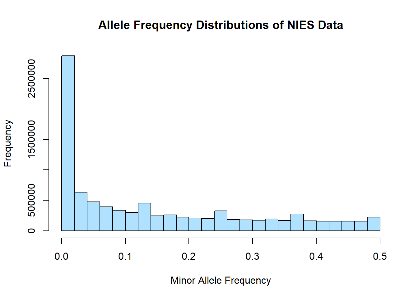

16. Apply filter for missing genotypes

plink1.9 --bfile merged_nies --mind 0.05 --geno 0.01 --make-bed --out nies_miss_filtered

Output: - 2 individuals removed (359 individuals remain) - 3,160,490 variants removed (5,992,268 variants remain) - total genotyping rate = 97.70%

Although this has significantly improved, two individuals were still removed and there is still a substantial number of variants being filtered out.

17. Apply a less stringent filter

plink1.9 --bfile merged_nies --mind 0.1 --geno 0.05 --make-bed --out nies_miss_filtered

Output: - 0 individuals removed - 1,096,020 variants removed (8,056,738 variants remain)

18. Check allele frequency

plink1.9 --bfile nies_miss_filtered --freq --out plink_output/nies_merged_snp_freq

Output: - 361 individuals loaded - 8,056,738 variants - total genotyping rate = 99.24%

19. Load allele frequency file

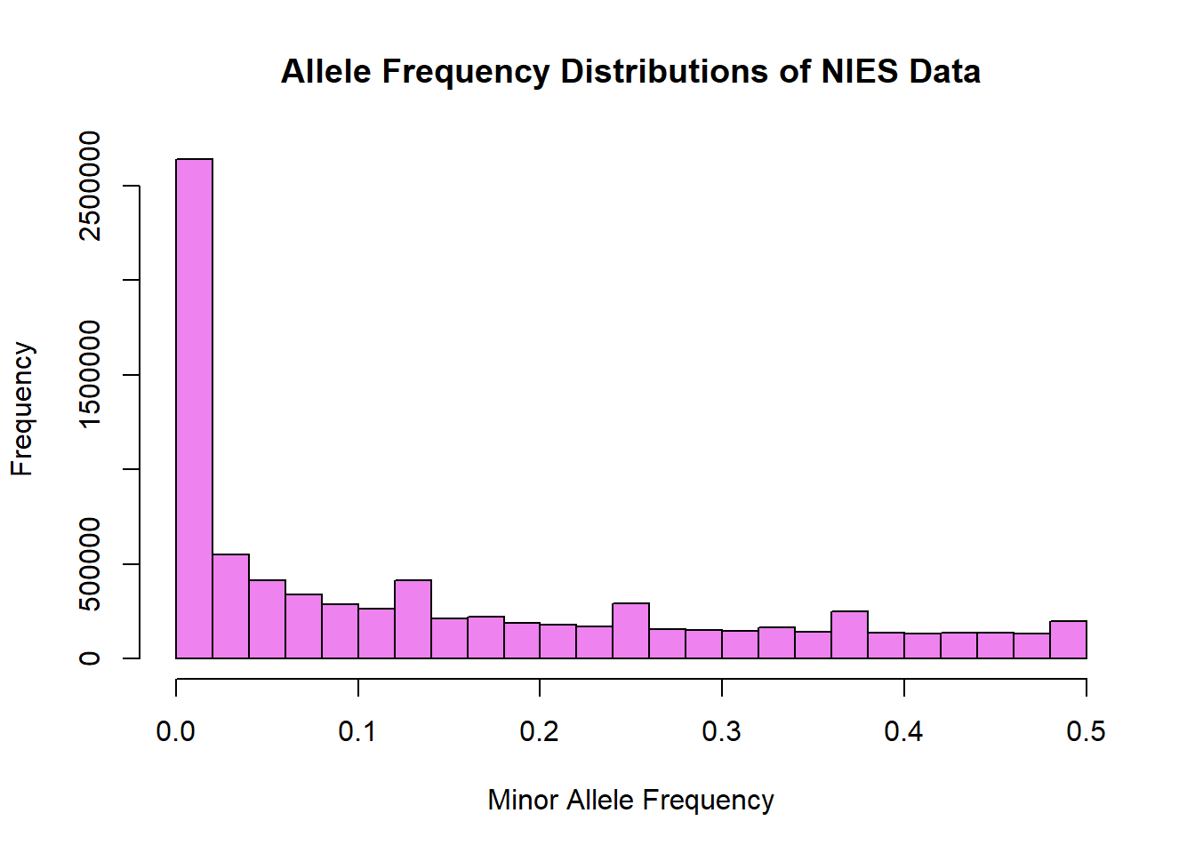
nies_merged_snp_freq <- read.table('C:/Users/Martha/Documents/Honours/Project/honours.project/Data/plink_output/nies_merged_snp_freq.frq', header = T)

20. Generate histogram for allele frequency distribution

hist(nies_merged_snp_freq$MAF, main = "Allele Frequency Distributions of NIES Data", xlab = "Minor Allele Frequency", xlim = c(0.0, 0.5), col = "violet")

Troubleshooting missing genotype filtering