| tags: [ Gaston Genomic Data R PLINK Heritability ] categories: [Coding Experiments ]
Using gaston for estimating heritability-1
Introduction
The genetic relationship matrix generated from the previous exercise contains values that signify the degree of relatedness between the individuals. This will allow me to estimate the heritability of the traits and principal components identified in the first objective.
To recap this concept, traits can vary among individuals due to environmental and genetic factors. Estimating the heritability of a trait means determining the proportion of variance that can be attributed to genetics (https://www.nature.com/scitable/topicpage/estimating-trait-heritability-46889). The relationship matrix is used to account for the degree of relatedness between the individuals when considering phenotypic variance. This is how heritabiity estimates are calculated.
Methods and Results
1. Load imputed phenotypic data
imputed_phen_data <- read.csv('C:/Users/Martha/Documents/Honours/Project/honours.project/imputed_phenotypic_data_uvaf.csv', header = T)

head(imputed_phen_data)
## UUID R.Logmar.VA L.Logmar.VA R.Sph..pre.dilate. R.Cyl..pre.dilate.
## 1 219960 0.02 -0.04 0.25 0.00
## 2 313180 0.10 0.16 0.00 -0.75
## 3 314911 0.00 0.00 1.25 -1.25
## 4 111150 0.30 0.08 1.25 -0.25
## 5 363161 0.00 -0.10 1.25 -0.25
## 6 110460 0.24 0.36 4.00 -0.50
## R.Axis..pre.dilate. L.Sph..pre.dilate. L.Cyl..pre.dilate.
## 1 0 0.25 -0.50
## 2 28 -0.50 -0.25
## 3 148 1.25 -0.25
## 4 97 1.50 -0.50
## 5 37 1.25 -0.75
## 6 46 3.75 -0.75
## L.Axis..pre.dilate. R.K.value.H R.K.Value.H.Axis R.K.value.V
## 1 79 42.00000 2.0000 43.00000
## 2 164 41.25000 7.0000 42.25000
## 3 24 43.91437 145.9032 44.91517
## 4 81 44.75000 5.0000 45.00000
## 5 164 44.75000 0.0000 44.75000
## 6 180 42.00000 8.0000 43.25000
## R.K.value.V.Axis L.K.value.H L.K.value.H.Axis L.K.value.V
## 1 92.00000 42.50000 5.00000 43.50000
## 2 97.00000 41.50000 168.00000 42.00000
## 3 49.64518 44.06458 38.39706 44.88776
## 4 95.00000 45.00000 60.00000 45.25000
## 5 90.00000 44.25000 178.00000 44.75000
## 6 98.00000 42.25000 177.00000 43.25000
## L.K.value.V.Axis R.Pachimetry L.Pachimetry R.Axial.Length L.Axial.Length
## 1 95.0000 532 554 24.31 24.10
## 2 78.0000 608 612 25.02 25.21
## 3 137.2832 507 510 22.78 22.80
## 4 150.0000 560 559 23.02 22.98
## 5 88.0000 556 562 21.75 22.04
## 6 87.0000 498 501 23.06 23.17
## R.AC.Depth L.AC.Depth R.IOP.mmHg L.IOP.mmHg R.CDR L.CDR totaluvafmm
## 1 3.09 3.03 14 14 0.9 0.9 0.00000
## 2 3.38 3.92 16 15 0.9 0.7 74.40000
## 3 3.40 3.45 26 22 0.7 0.7 14.60000
## 4 3.00 2.85 14 14 0.2 0.2 1.90000
## 5 2.60 2.53 22 21 0.3 0.3 23.98903
## 6 2.94 3.04 18 20 0.6 0.6 1.000002. Load genomic data
merged_nies_fam <- read.table('C:/Users/Martha/Documents/Honours/Project/honours.project/Data/merged_nies_filtered.fam', header = F)

head(merged_nies_fam)
## V1 V2 V3 V4 V5 V6
## 1 1 110150 0 0 2 -9
## 2 1 110160 0 0 1 -9
## 3 1 110500 0 0 2 -9
## 4 1 110650 0 0 2 -9
## 5 1 110820 0 0 2 -9
## 6 1 111280 0 0 2 -93. Extract UUIDs in genomic data
geno_data_uuid <- merged_nies_fam$V24. Extract relevant phenotypic data based on genomic UUIDs
nies_pheno <- imputed_phen_data[imputed_phen_data$UUID %in% c(geno_data_uuid), ]
head(nies_pheno)
## UUID R.Logmar.VA L.Logmar.VA R.Sph..pre.dilate. R.Cyl..pre.dilate.
## 1 219960 0.02 -0.04 0.25 0.00
## 2 313180 0.10 0.16 0.00 -0.75
## 7 320511 -0.06 0.02 1.00 0.00
## 11 400011 -0.14 -0.10 0.75 -0.25
## 13 400013 0.30 0.30 1.50 -0.25
## 14 316131 0.08 0.26 2.00 -1.00
## R.Axis..pre.dilate. L.Sph..pre.dilate. L.Cyl..pre.dilate.
## 1 0 0.25 -0.50
## 2 28 -0.50 -0.25
## 7 0 1.25 -0.25
## 11 157 1.25 -0.50
## 13 82 1.75 -0.50
## 14 69 1.00 -1.00
## L.Axis..pre.dilate. R.K.value.H R.K.Value.H.Axis R.K.value.V
## 1 79 42.00 2 43.00
## 2 164 41.25 7 42.25
## 7 29 42.50 177 43.50
## 11 20 42.50 165 43.25
## 13 100 43.00 0 43.00
## 14 114 42.75 63 44.00
## R.K.value.V.Axis L.K.value.H L.K.value.H.Axis L.K.value.V
## 1 92 42.50 5 43.50
## 2 97 41.50 168 42.00
## 7 87 42.00 170 42.50
## 11 75 42.75 17 43.25
## 13 90 42.75 111 43.00
## 14 153 43.00 115 43.50
## L.K.value.V.Axis R.Pachimetry L.Pachimetry R.Axial.Length
## 1 95 532 554 24.31
## 2 78 608 612 25.02
## 7 80 499 512 23.37
## 11 107 602 601 23.32
## 13 21 552 550 22.93
## 14 25 583 588 23.49
## L.Axial.Length R.AC.Depth L.AC.Depth R.IOP.mmHg L.IOP.mmHg R.CDR L.CDR
## 1 24.10 3.09 3.03 14 14 0.9 0.9
## 2 25.21 3.38 3.92 16 15 0.9 0.7
## 7 23.65 3.29 3.08 17 18 0.4 0.4
## 11 23.34 3.81 3.83 15 17 0.6 0.6
## 13 22.70 3.22 3.13 18 18 0.4 0.4
## 14 23.54 3.24 3.04 12 12 0.3 0.3
## totaluvafmm
## 1 0.0
## 2 74.4
## 7 27.5
## 11 47.0
## 13 20.1
## 14 12.9I thought that all 359 individuals would have phenotypic data. However, only 346 individuals were extracted, indicating that there are 346 individuals with phenotypic and genomic data. This is most likely because I removed individuals that were <17 years old.
5. Isolate UUIDs of phenotypic data
pheno_data_uuid <- nies_pheno$UUIDwrite.table(pheno_data_uuid, 'C:/Users/Martha/Documents/Honours/honours.project/Data/filtered_pheno_uuid.txt', row.names = F, col.names = F, quote = F)6. Extract genomic data for individuals with phenotypic data
plink1.9 --bfile merged_nies_filtered --keep filtered_pheno_uuid2.txt --make-bed --out merged_nies_genoNote: I added a family ID column to the text file as PLINK only recognises ID files when they have family and individual IDs.
Output:
346 individuals remain
13 individuals removed
3,910,077 variants remain
7. Re-order samples in genomic data set based on order of UUIDs of phenotypic data set
plink1.9 --bfile merged_nies_geno --indiv-sort f filtered_pheno_uuid2.txt --make-bed --out merged_nies_genoThe samples have to be re-ordered to be the same as the phenotypic data for estimating heritability.
8. Run PCA on this new filtered data set
plink1.9 --bfile merged_nies_geno --pca 120 var-wts --out plink_output/nies_geno_pcaPCA and generating GRM have to be repeated for this new data set as it contains less individuals compared to the last data set.
9. Load eigenvalue file and generate screeplot.
nies_geno_eigenval <- read.table('C:/Users/Martha/Documents/Honours/Project/honours.project/Data/plink_output/nies_geno_pca.eigenval', header = F)

barplot(nies_geno_eigenval$V1,
        names.arg = 1:nrow(nies_geno_eigenval),
        main = "NIES PCA Eigenvalue",
        xlab = "Principal Components",
        ylab = "Eigenvalue",
        col ="lightskyblue2")
lines(x = 1:nrow(nies_geno_eigenval), nies_geno_eigenval$V1,
      type = "b", pch = 19, col = "red")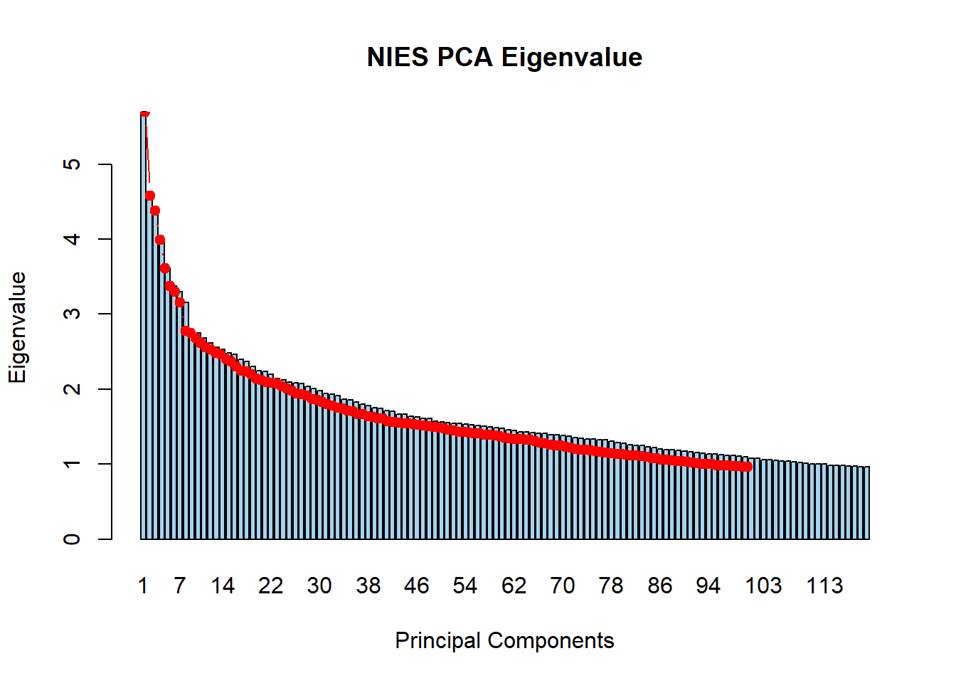
There are 112 PCs with an eigenvalue >1.
10. Load eigenvector files
nies_geno_eigenvec <- read.table('C:/Users/Martha/Documents/Honours/Project/honours.project/Data/plink_output/nies_geno_pca.eigenvec', header = F)11. Generate eigenvector plots
plot(nies_geno_eigenvec$V3, nies_geno_eigenvec$V4, xlab = "PC1", ylab = "PC2", main = "PC1 vs PC2 eigenvectors") 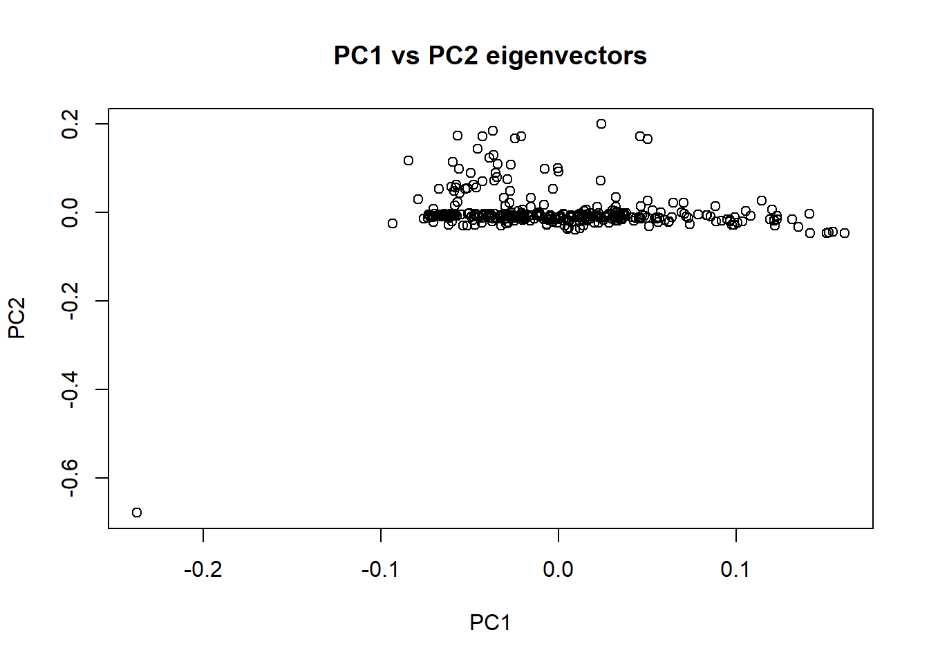
plot(nies_geno_eigenvec$V4, nies_geno_eigenvec$V5, xlab = "PC2", ylab = "PC3", main = "PC2 vs PC3 eigenvectors")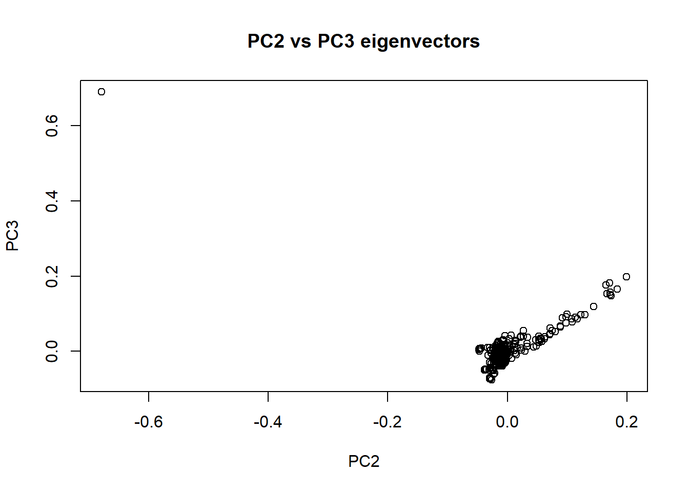
The outlier individual is still present in these plots. I need to identify and remove the individual from the data set. Rod speculated that this outlier may have been caused by a technical error. Since the individuals sequenced are part of the core pedigree, there should only be a single cluster of individuals in these plots. Therefore, having an individual that is significantly further away from the cluster is unusual.
11a. Add labels to the plot to identify the outlier
require(ggplot2)## Loading required package: ggplot2pc1Vpc2 <- data.frame(PC1 = nies_geno_eigenvec$V3, PC2 = nies_geno_eigenvec$V4, names = nies_geno_eigenvec$V2)
ggplot(pc1Vpc2, aes(PC1, PC2)) + geom_point() + geom_text(aes(label=names))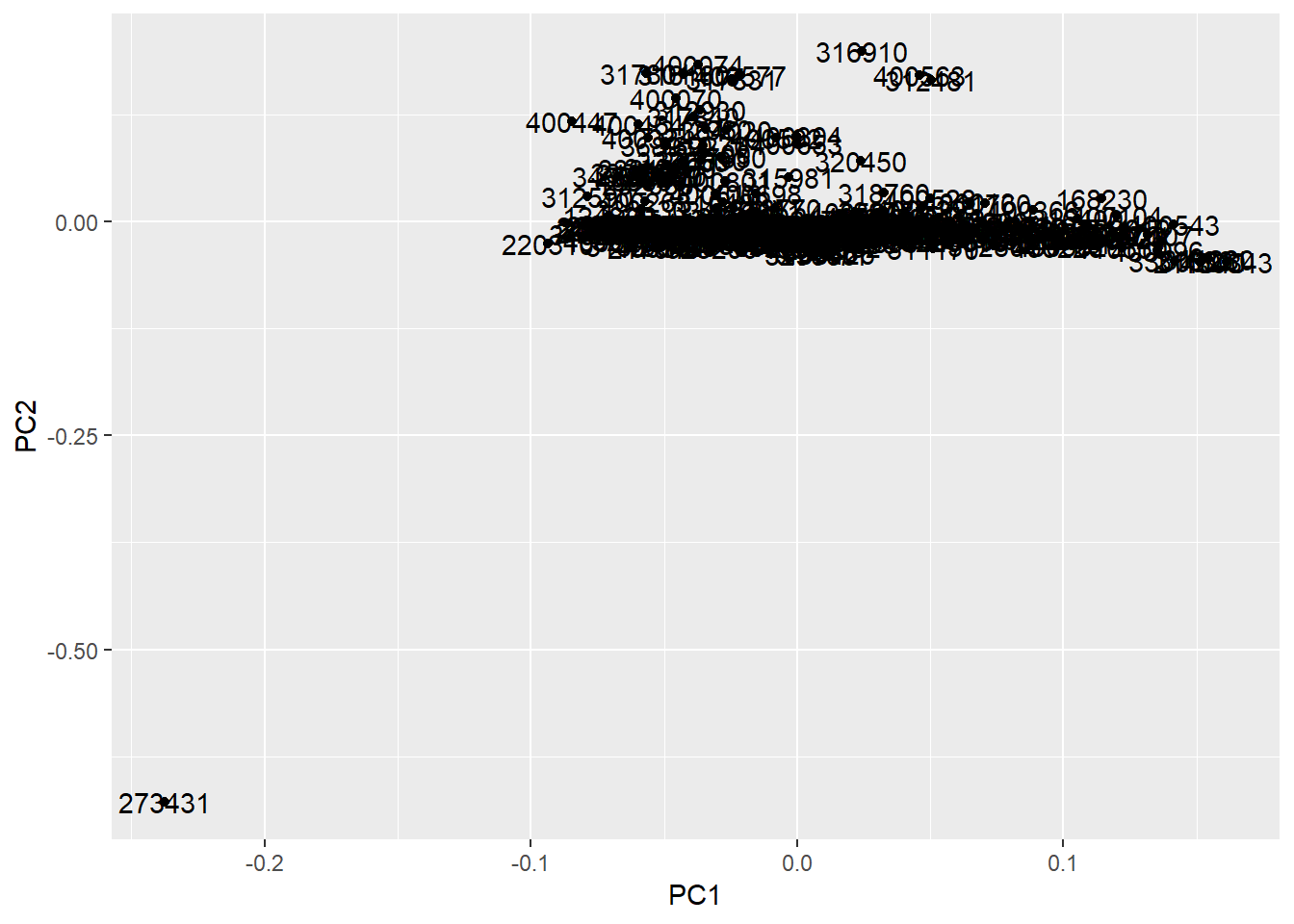
The outlier’s UUID is 273431.
12. Remove outlier individual from phenotypic and genomic data sets.
Check that the individuals are still in the same order after removing the data set.
- Removed UUID 273431 from the ID list
Remove individual from genomic data set
plink1.9 --bfile merged_nies_geno --keep filtered_pheno_uuid3 --make-bed --out merged_nies_geno_210818merged_nies_fam_210818 <- read.table('C:/Users/Martha/Documents/Honours/Project/honours.project/Data/merged_nies/merged_nies_geno_210818.fam', header = F)
head(merged_nies_fam_210818)## V1 V2 V3 V4 V5 V6
## 1 1 219960 0 0 1 -9
## 2 1 313180 0 0 1 -9
## 3 1 320511 0 0 2 -9
## 4 1 400011 0 0 1 -9
## 5 1 400013 0 0 1 -9
## 6 1 316131 0 0 2 -9geno_data_uuid2 <- merged_nies_fam_210818$V2Remove individual from phenotypic data set
nies_pheno_210818 <- nies_pheno[nies_pheno$UUID %in% c(geno_data_uuid2), ]
head(nies_pheno_210818)
## UUID R.Logmar.VA L.Logmar.VA R.Sph..pre.dilate. R.Cyl..pre.dilate.
## 1 219960 0.02 -0.04 0.25 0.00
## 2 313180 0.10 0.16 0.00 -0.75
## 7 320511 -0.06 0.02 1.00 0.00
## 11 400011 -0.14 -0.10 0.75 -0.25
## 13 400013 0.30 0.30 1.50 -0.25
## 14 316131 0.08 0.26 2.00 -1.00
## R.Axis..pre.dilate. L.Sph..pre.dilate. L.Cyl..pre.dilate.
## 1 0 0.25 -0.50
## 2 28 -0.50 -0.25
## 7 0 1.25 -0.25
## 11 157 1.25 -0.50
## 13 82 1.75 -0.50
## 14 69 1.00 -1.00
## L.Axis..pre.dilate. R.K.value.H R.K.Value.H.Axis R.K.value.V
## 1 79 42.00 2 43.00
## 2 164 41.25 7 42.25
## 7 29 42.50 177 43.50
## 11 20 42.50 165 43.25
## 13 100 43.00 0 43.00
## 14 114 42.75 63 44.00
## R.K.value.V.Axis L.K.value.H L.K.value.H.Axis L.K.value.V
## 1 92 42.50 5 43.50
## 2 97 41.50 168 42.00
## 7 87 42.00 170 42.50
## 11 75 42.75 17 43.25
## 13 90 42.75 111 43.00
## 14 153 43.00 115 43.50
## L.K.value.V.Axis R.Pachimetry L.Pachimetry R.Axial.Length
## 1 95 532 554 24.31
## 2 78 608 612 25.02
## 7 80 499 512 23.37
## 11 107 602 601 23.32
## 13 21 552 550 22.93
## 14 25 583 588 23.49
## L.Axial.Length R.AC.Depth L.AC.Depth R.IOP.mmHg L.IOP.mmHg R.CDR L.CDR
## 1 24.10 3.09 3.03 14 14 0.9 0.9
## 2 25.21 3.38 3.92 16 15 0.9 0.7
## 7 23.65 3.29 3.08 17 18 0.4 0.4
## 11 23.34 3.81 3.83 15 17 0.6 0.6
## 13 22.70 3.22 3.13 18 18 0.4 0.4
## 14 23.54 3.24 3.04 12 12 0.3 0.3
## totaluvafmm
## 1 0.0
## 2 74.4
## 7 27.5
## 11 47.0
## 13 20.1
## 14 12.913. Re-run PCA on genomic data set
plink1.9 --bfile merged_nies_pheno_210818 --pca 120 var-wts --out plink_output/nies_pca_21081814. Load eigenvalue file and generate screeplot
nies_eigenval_210818 <- read.table('C:/Users/Martha/Documents/Honours/Project/honours.project/Data/plink_output/nies_pca_210818.eigenval', header = F)

barplot(nies_eigenval_210818$V1,
        names.arg = 1:nrow(nies_eigenval_210818),
        main = "NIES PCA Eigenvalue",
        xlab = "Principal Components",
        ylab = "Eigenvalue",
        col ="lightskyblue2")
lines(x = 1:nrow(nies_eigenval_210818), nies_eigenval_210818$V1,
      type = "b", pch = 19, col = "red")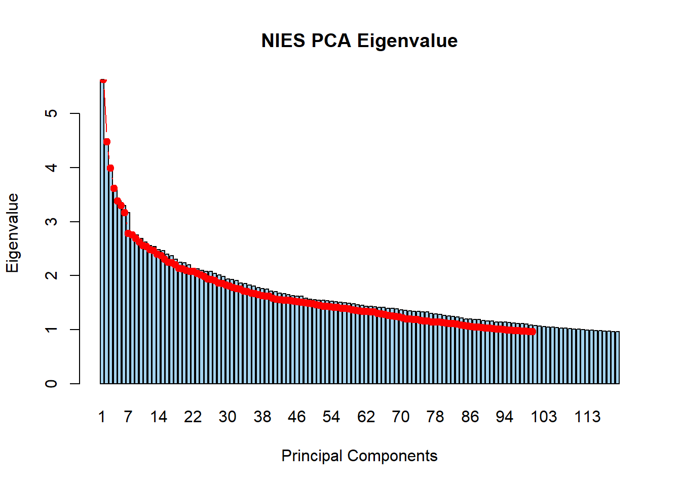
16. Load eigenvector file and check that outlier is not present in PCA plots
nies_eigenvec_210818 <- read.table('C:/Users/Martha/Documents/Honours/Project/honours.project/Data/plink_output/nies_pca_210818.eigenvec', header = F)

plot(nies_eigenvec_210818$V3, nies_eigenvec_210818$V4, xlab = "PC1", ylab = "PC2", main = "PC1 vs PC2 eigenvectors")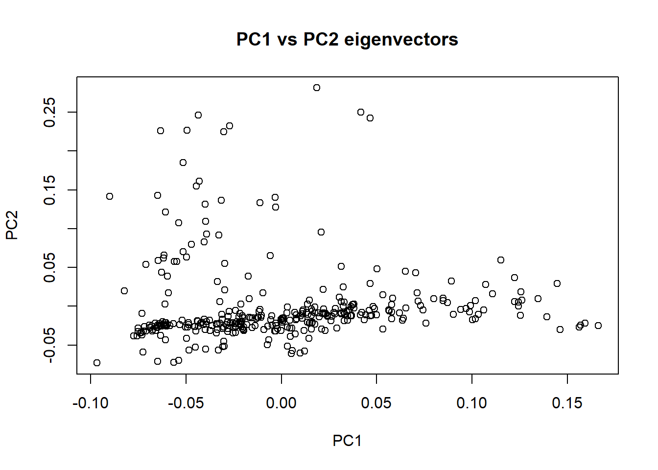
17. Load genomic data
require(gaston)## Loading required package: gaston## Loading required package: Rcpp## Loading required package: RcppParallel##
## Attaching package: 'RcppParallel'## The following object is masked from 'package:Rcpp':
##
## LdFlags## Gaston set number of threads to 2. Use setThreadOptions() to modify this.##
## Attaching package: 'gaston'## The following object is masked from 'package:stats':
##
## sigma## The following objects are masked from 'package:base':
##
## cbind, rbindmerged_nies_210818 <- read.bed.matrix("C:/Users/Martha/Documents/Honours/Project/honours.project/Data/merged_nies/merged_nies_geno_210818.bed")## Reading C:/Users/Martha/Documents/Honours/Project/honours.project/Data/merged_nies/merged_nies_geno_210818.fam
## Reading C:/Users/Martha/Documents/Honours/Project/honours.project/Data/merged_nies/merged_nies_geno_210818.bim
## Reading C:/Users/Martha/Documents/Honours/Project/honours.project/Data/merged_nies/merged_nies_geno_210818.bed
## ped stats and snps stats have been set.
## 'p' has been set.
## 'mu' and 'sigma' have been set.18. Generate GRM using gaston
Ensure that the individuals are in the same order as the phenotypic and genomic data.
merged_nies_GRM <- GRM(merged_nies_210818)19. Compute eigen decomposition
merged_nies_eiK <- eigen(merged_nies_GRM)20. Deal with small negative eigenvalues
merged_nies_eiK$values[ merged_nies_eiK$values < 0] <- 018. Perform PCA on GRM
merged_nies_PC <- sweep(merged_nies_eiK$vectors, 2, sqrt(merged_nies_eiK$values), "*")19. Plot eigenvector values from PCA of the GRM
plot(merged_nies_PC[,1], merged_nies_PC[,2], xlab = "PC1", ylab = "PC2", main = "GRM PC1 vs PC2") 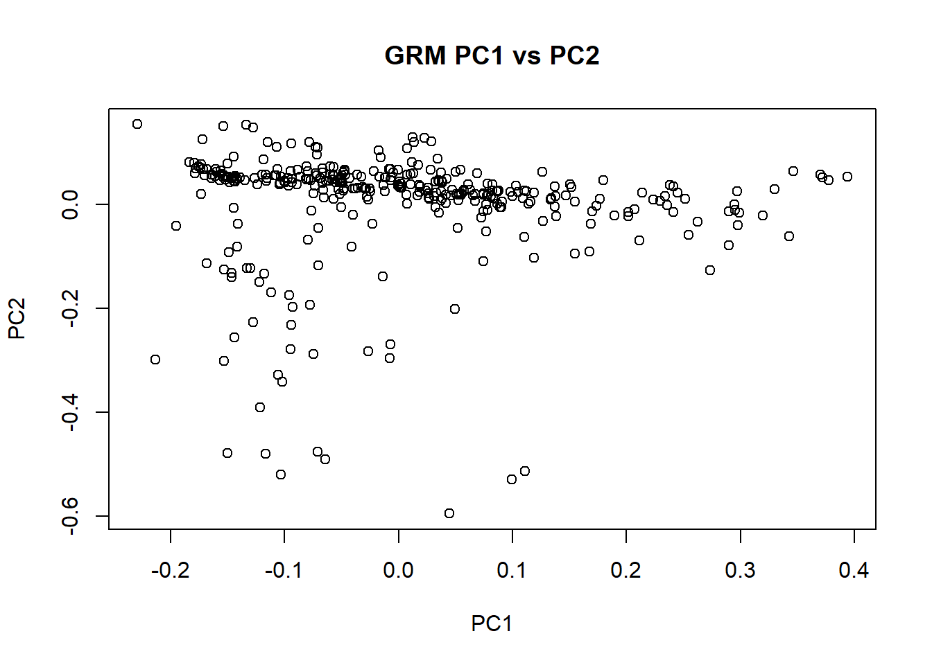
20. Test lmm.diago() function (gaston)
Y <- nies_pheno_210818$R.K.value.H
fit <- lmm.diago(Y, eigenK = merged_nies_eiK)
## Optimization in interval [0, 1]
## Optimizing with p = 0
## [Iteration 1] Current point = 0 df = 41.4731
## [Iteration 2] Current point = 0.231523 df = 18.3374
## [Iteration 3] Current point = 0.518644 df = 0.833621
## [Iteration 4] Current point = 0.530343 df = -0.0125581
## [Iteration 5] Current point = 0.530172 df = -2.86236e-006h^2 of horizontal R K-value = 53.01% (?)
21. Repeat for all phenotypic variables
for (i in 2:ncol(nies_pheno_210818)){
fit <- lmm.diago(nies_pheno_210818[,i], eigenK = merged_nies_eiK)}## Optimization in interval [0, 1]
## Optimizing with p = 0
## [Iteration 1] Current point = 0 df = -2.2559
## [Iteration 1] maximum at min = 0
## Optimization in interval [0, 1]
## Optimizing with p = 0
## [Iteration 1] Current point = 0 df = -16.655
## [Iteration 1] maximum at min = 0
## Optimization in interval [0, 1]
## Optimizing with p = 0
## [Iteration 1] Current point = 0 df = -9.57183
## [Iteration 1] maximum at min = 0
## Optimization in interval [0, 1]
## Optimizing with p = 0
## [Iteration 1] Current point = 0 df = 28.3745
## [Iteration 2] Current point = 0.484116 df = 4.41849
## [Iteration 3] Current point = 0.550692 df = -0.406865
## [Iteration 4] Current point = 0.545563 df = -0.00300791
## [Iteration 5] Current point = 0.545525 df = -1.66267e-007
## Optimization in interval [0, 1]
## Optimizing with p = 0
## [Iteration 1] Current point = 0 df = 2.08593
## [Iteration 2] Current point = 0.0336347 df = 0.117014
## [Iteration 3] Current point = 0.0357434 df = 0.000347961
## [Iteration 4] Current point = 0.0357497 df = 3.06179e-009
## Optimization in interval [0, 1]
## Optimizing with p = 0
## [Iteration 1] Current point = 0 df = -10.2621
## [Iteration 1] maximum at min = 0
## Optimization in interval [0, 1]
## Optimizing with p = 0
## [Iteration 1] Current point = 0 df = -7.03848
## [Iteration 1] maximum at min = 0
## Optimization in interval [0, 1]
## Optimizing with p = 0
## [Iteration 1] Current point = 0 df = 7.05039
## [Iteration 2] Current point = 0.0729428 df = 1.33525
## [Iteration 3] Current point = 0.0934138 df = 0.0496894
## [Iteration 4] Current point = 0.0942343 df = 6.77127e-005
## Optimization in interval [0, 1]
## Optimizing with p = 0
## [Iteration 1] Current point = 0 df = 41.4731
## [Iteration 2] Current point = 0.231523 df = 18.3374
## [Iteration 3] Current point = 0.518644 df = 0.833621
## [Iteration 4] Current point = 0.530343 df = -0.0125581
## [Iteration 5] Current point = 0.530172 df = -2.86236e-006
## Optimization in interval [0, 1]
## Optimizing with p = 0
## [Iteration 1] Current point = 0 df = -9.56967
## [Iteration 1] maximum at min = 0
## Optimization in interval [0, 1]
## Optimizing with p = 0
## [Iteration 1] Current point = 0 df = 49.5036
## [Iteration 2] Current point = 0.266942 df = 26.2542
## [Iteration 3] Current point = 0.821788 df = -9.32438
## [Iteration 4] Current point = 0.775858 df = -1.952
## [Iteration 5] Current point = 0.760616 df = -0.116259
## [Iteration 6] Current point = 0.75959 df = -0.000450576
## [Iteration 7] Current point = 0.759586 df = -6.78389e-009
## Optimization in interval [0, 1]
## Optimizing with p = 0
## [Iteration 1] Current point = 0 df = -14.4913
## [Iteration 1] maximum at min = 0
## Optimization in interval [0, 1]
## Optimizing with p = 0
## [Iteration 1] Current point = 0 df = 35.3151
## [Iteration 2] Current point = 0.1702 df = 13.7743
## [Iteration 3] Current point = 0.334479 df = 1.91493
## [Iteration 4] Current point = 0.363073 df = -0.00294203
## [Iteration 5] Current point = 0.363029 df = -2.35821e-008
## Optimization in interval [0, 1]
## Optimizing with p = 0
## [Iteration 1] Current point = 0 df = 0.484426
## [Iteration 2] Current point = 0.0064578 df = 0.0122138
## [Iteration 3] Current point = 0.0066291 df = 7.97164e-006
## Optimization in interval [0, 1]
## Optimizing with p = 0
## [Iteration 1] Current point = 0 df = 47.5036
## [Iteration 2] Current point = 0.21944 df = 22.4879
## [Iteration 3] Current point = 0.552683 df = 3.68487
## [Iteration 4] Current point = 0.614956 df = -0.223631
## [Iteration 5] Current point = 0.61162 df = -0.000894753
## [Iteration 6] Current point = 0.611607 df = -1.43198e-008
## Optimization in interval [0, 1]
## Optimizing with p = 0
## [Iteration 1] Current point = 0 df = -5.823
## [Iteration 1] maximum at min = 0
## Optimization in interval [0, 1]
## Optimizing with p = 0
## [Iteration 1] Current point = 0 df = 38.2559
## [Iteration 2] Current point = 0.27791 df = 16.0916
## [Iteration 3] Current point = 0.570976 df = 0.713281
## [Iteration 4] Current point = 0.583485 df = -0.00665774
## [Iteration 5] Current point = 0.58337 df = -5.94581e-007
## Optimization in interval [0, 1]
## Optimizing with p = 0
## [Iteration 1] Current point = 0 df = 40.2764
## [Iteration 2] Current point = 0.310726 df = 16.9307
## [Iteration 3] Current point = 0.640107 df = 0.435845
## [Iteration 4] Current point = 0.647777 df = -0.00294086
## [Iteration 5] Current point = 0.647726 df = -1.34981e-007
## Optimization in interval [0, 1]
## Optimizing with p = 0
## [Iteration 1] Current point = 0 df = 23.1767
## [Iteration 2] Current point = 0.197614 df = 7.99998
## [Iteration 3] Current point = 0.339062 df = 0.598113
## [Iteration 4] Current point = 0.350965 df = 7.42912e-005
## Optimization in interval [0, 1]
## Optimizing with p = 0
## [Iteration 1] Current point = 0 df = 23.1579
## [Iteration 2] Current point = 0.183926 df = 8.23487
## [Iteration 3] Current point = 0.324513 df = 0.719946
## [Iteration 4] Current point = 0.338682 df = 0.000540716
## [Iteration 5] Current point = 0.338693 df = 5.47118e-012
## Optimization in interval [0, 1]
## Optimizing with p = 0
## [Iteration 1] Current point = 0 df = 27.2665
## [Iteration 2] Current point = 0.18723 df = 8.27687
## [Iteration 3] Current point = 0.296964 df = 0.659801
## [Iteration 4] Current point = 0.307044 df = 0.00182903
## [Iteration 5] Current point = 0.307072 df = 1.20226e-008
## Optimization in interval [0, 1]
## Optimizing with p = 0
## [Iteration 1] Current point = 0 df = 25.4208
## [Iteration 2] Current point = 0.180651 df = 7.2106
## [Iteration 3] Current point = 0.274918 df = 0.536193
## [Iteration 4] Current point = 0.282972 df = 0.00194078
## [Iteration 5] Current point = 0.283001 df = 2.39764e-008
## Optimization in interval [0, 1]
## Optimizing with p = 0
## [Iteration 1] Current point = 0 df = 19.0563
## [Iteration 2] Current point = 0.147446 df = 6.12048
## [Iteration 3] Current point = 0.24176 df = 0.503822
## [Iteration 4] Current point = 0.250745 df = 0.00152377
## [Iteration 5] Current point = 0.250772 df = 1.21091e-008
## Optimization in interval [0, 1]
## Optimizing with p = 0
## [Iteration 1] Current point = 0 df = 19.565
## [Iteration 2] Current point = 0.131325 df = 5.87129
## [Iteration 3] Current point = 0.206538 df = 0.500194
## [Iteration 4] Current point = 0.214074 df = 0.00268863
## [Iteration 5] Current point = 0.214115 df = 7.4301e-008
## Optimization in interval [0, 1]
## Optimizing with p = 0
## [Iteration 1] Current point = 0 df = 72.9477
## [Iteration 2] Current point = 0.158165 df = 35.0727
## [Iteration 3] Current point = 0.434828 df = 12.9756
## [Iteration 4] Current point = 0.647277 df = -1.20794
## [Iteration 5] Current point = 0.632241 df = -0.0237355
## [Iteration 6] Current point = 0.631934 df = -9.17477e-006
## Optimization in interval [0, 1]
## Optimizing with p = 0
## [Iteration 1] Current point = 0 df = 75.6479
## [Iteration 2] Current point = 0.147316 df = 35.2271
## [Iteration 3] Current point = 0.385568 df = 13.2911
## [Iteration 4] Current point = 0.589986 df = 0.309687
## [Iteration 5] Current point = 0.5945 df = -0.00121467
## [Iteration 6] Current point = 0.594482 df = -1.89248e-008
## Optimization in interval [0, 1]
## Optimizing with p = 0
## [Iteration 1] Current point = 0 df = 24.1626
## [Iteration 2] Current point = 0.244014 df = 8.88222
## [Iteration 3] Current point = 0.432413 df = 0.131632
## [Iteration 4] Current point = 0.435111 df = -0.00021394922. Include two principal components for estimating heritability
for (i in 2:ncol(nies_pheno_210818)){
  fit <- lmm.diago(nies_pheno_210818[,i], eigenK = merged_nies_eiK, p = 2)}
## Optimization in interval [0, 1]
## Optimizing with p = 2
## [Iteration 1] Current point = 0 df = -7.11013
## [Iteration 1] maximum at min = 0
## Optimization in interval [0, 1]
## Optimizing with p = 2
## [Iteration 1] Current point = 0 df = -13.3561
## [Iteration 1] maximum at min = 0
## Optimization in interval [0, 1]
## Optimizing with p = 2
## [Iteration 1] Current point = 0 df = -8.19357
## [Iteration 1] maximum at min = 0
## Optimization in interval [0, 1]
## Optimizing with p = 2
## [Iteration 1] Current point = 0 df = 28.7103
## [Iteration 2] Current point = 0.599149 df = -3.46492
## [Iteration 3] Current point = 0.561391 df = -0.198617
## [Iteration 4] Current point = 0.558957 df = -0.000713875
## [Iteration 5] Current point = 0.558948 df = -9.27375e-009
## Optimization in interval [0, 1]
## Optimizing with p = 2
## [Iteration 1] Current point = 0 df = 3.78121
## [Iteration 2] Current point = 0.0614073 df = 0.309897
## [Iteration 3] Current point = 0.0673109 df = 0.00175775
## [Iteration 4] Current point = 0.0673448 df = 5.52169e-008
## Optimization in interval [0, 1]
## Optimizing with p = 2
## [Iteration 1] Current point = 0 df = -10.5435
## [Iteration 1] maximum at min = 0
## Optimization in interval [0, 1]
## Optimizing with p = 2
## [Iteration 1] Current point = 0 df = -4.78203
## [Iteration 1] maximum at min = 0
## Optimization in interval [0, 1]
## Optimizing with p = 2
## [Iteration 1] Current point = 0 df = 6.30518
## [Iteration 2] Current point = 0.0910141 df = 0.794675
## [Iteration 3] Current point = 0.105783 df = 0.011704
## [Iteration 4] Current point = 0.106007 df = 2.46312e-006
## Optimization in interval [0, 1]
## Optimizing with p = 2
## [Iteration 1] Current point = 0 df = 29.269
## [Iteration 2] Current point = 0.347647 df = 9.62902
## [Iteration 3] Current point = 0.542008 df = -1.62963
## [Iteration 4] Current point = 0.519432 df = -0.0548232
## [Iteration 5] Current point = 0.518619 df = -6.32935e-005
## Optimization in interval [0, 1]
## Optimizing with p = 2
## [Iteration 1] Current point = 0 df = -7.36338
## [Iteration 1] maximum at min = 0
## Optimization in interval [0, 1]
## Optimizing with p = 2
## [Iteration 1] Current point = 0 df = 34.8249
## [Iteration 2] Current point = 0.531217 df = 14.0813
## [Iteration 3] Current point = 0.879187 df = -27.5399
## [Iteration 4] Current point = 0.823716 df = -9.91648
## [Iteration 5] Current point = 0.775494 df = -2.20567
## [Iteration 6] Current point = 0.757915 df = -0.152536
## [Iteration 7] Current point = 0.756513 df = -0.000811872
## [Iteration 8] Current point = 0.756506 df = -2.31775e-008
## Optimization in interval [0, 1]
## Optimizing with p = 2
## [Iteration 1] Current point = 0 df = -11.3499
## [Iteration 1] maximum at min = 0
## Optimization in interval [0, 1]
## Optimizing with p = 2
## [Iteration 1] Current point = 0 df = 14.3799
## [Iteration 2] Current point = 0.263585 df = 1.54924
## [Iteration 3] Current point = 0.295381 df = -0.0212347
## [Iteration 4] Current point = 0.294957 df = -4.56719e-006
## Optimization in interval [0, 1]
## Optimizing with p = 2
## [Iteration 1] Current point = 0 df = -0.187161
## [Iteration 1] maximum at min = 0
## Optimization in interval [0, 1]
## Optimizing with p = 2
## [Iteration 1] Current point = 0 df = 29.0126
## [Iteration 2] Current point = 0.435271 df = 8.12837
## [Iteration 3] Current point = 0.613725 df = -1.21958
## [Iteration 4] Current point = 0.59433 df = -0.0309852
## [Iteration 5] Current point = 0.593811 df = -2.01423e-005
## Optimization in interval [0, 1]
## Optimizing with p = 2
## [Iteration 1] Current point = 0 df = -2.94506
## [Iteration 1] maximum at min = 0
## Optimization in interval [0, 1]
## Optimizing with p = 2
## [Iteration 1] Current point = 0 df = 36.5065
## [Iteration 2] Current point = 0.356508 df = 12.8279
## [Iteration 3] Current point = 0.610013 df = -0.571562
## [Iteration 4] Current point = 0.600536 df = -0.0047655
## [Iteration 5] Current point = 0.600456 df = -3.27571e-007
## Optimization in interval [0, 1]
## Optimizing with p = 2
## [Iteration 1] Current point = 0 df = 40.347
## [Iteration 2] Current point = 0.363064 df = 15.4634
## [Iteration 3] Current point = 0.677099 df = -0.587165
## [Iteration 4] Current point = 0.667423 df = -0.00565348
## [Iteration 5] Current point = 0.667328 df = -5.21474e-007
## Optimization in interval [0, 1]
## Optimizing with p = 2
## [Iteration 1] Current point = 0 df = 21.8958
## [Iteration 2] Current point = 0.254171 df = 5.84146
## [Iteration 3] Current point = 0.3687 df = 0.125045
## [Iteration 4] Current point = 0.37121 df = -5.02903e-005
## Optimization in interval [0, 1]
## Optimizing with p = 2
## [Iteration 1] Current point = 0 df = 20.5946
## [Iteration 2] Current point = 0.243888 df = 5.45003
## [Iteration 3] Current point = 0.351788 df = 0.10615
## [Iteration 4] Current point = 0.353935 df = -3.52901e-005
## Optimization in interval [0, 1]
## Optimizing with p = 2
## [Iteration 1] Current point = 0 df = 25.019
## [Iteration 2] Current point = 0.208385 df = 6.76504
## [Iteration 3] Current point = 0.307491 df = 0.337584
## [Iteration 4] Current point = 0.312871 df = 0.000239402
## Optimization in interval [0, 1]
## Optimizing with p = 2
## [Iteration 1] Current point = 0 df = 24.4286
## [Iteration 2] Current point = 0.198858 df = 6.34809
## [Iteration 3] Current point = 0.288122 df = 0.349883
## [Iteration 4] Current point = 0.293561 df = 0.000614758
## [Iteration 5] Current point = 0.293571 df = 1.79782e-009
## Optimization in interval [0, 1]
## Optimizing with p = 2
## [Iteration 1] Current point = 0 df = 17.157
## [Iteration 2] Current point = 0.18723 df = 4.28128
## [Iteration 3] Current point = 0.263656 df = 0.122049
## [Iteration 4] Current point = 0.265935 df = 1.29855e-005
## Optimization in interval [0, 1]
## Optimizing with p = 2
## [Iteration 1] Current point = 0 df = 15.7871
## [Iteration 2] Current point = 0.164015 df = 3.26658
## [Iteration 3] Current point = 0.21526 df = 0.0952811
## [Iteration 4] Current point = 0.216838 df = 5.61709e-005
## Optimization in interval [0, 1]
## Optimizing with p = 2
## [Iteration 1] Current point = 0 df = 33.0992
## [Iteration 2] Current point = 0.327339 df = 13.6128
## [Iteration 3] Current point = 0.632864 df = -2.41685
## [Iteration 4] Current point = 0.598798 df = -0.117288
## [Iteration 5] Current point = 0.596974 df = -0.000289291
## [Iteration 6] Current point = 0.596969 df = -1.76379e-009
## Optimization in interval [0, 1]
## Optimizing with p = 2
## [Iteration 1] Current point = 0 df = 30.6574
## [Iteration 2] Current point = 0.2758 df = 12.4104
## [Iteration 3] Current point = 0.5439 df = -0.185709
## [Iteration 4] Current point = 0.540475 df = -0.000632608
## [Iteration 5] Current point = 0.540463 df = -7.32253e-009
## Optimization in interval [0, 1]
## Optimizing with p = 2
## [Iteration 1] Current point = 0 df = 24.2256
## [Iteration 2] Current point = 0.303903 df = 7.32815
## [Iteration 3] Current point = 0.464196 df = -0.252431
## [Iteration 4] Current point = 0.459249 df = -0.000927276
## [Iteration 5] Current point = 0.459231 df = -1.23407e-008The output of this last step contains the narrow sense heritability estimates for each of the 27 variables in the phenotypic data set and the corresponding degrees of freedom. (need to add labels but it is in order of the variables as listed in the spreadsheet)
When interpreting the results, does the last iteration indicate the heritability estimate? Why are there varying numbers of iterations for the variables? For the variables where there is only 1 iteration and it says maximum at min = 0, how is this interpreted? How do I estimate the heritability for the principal components?